Species diversity is affected by resources, habitat diversity, keystone species, and disturbance
We have seen that communities differ in the number of species they contain, but we have not yet addressed the more fundamental question of why they differ. On a global scale, there is great variation in the number of species found in different locations. For example, naturalists have known for centuries that more species live in tropical regions than in temperate or boreal zones. We will discuss global patterns of species richness in later chapters and consider the effects of long-term processes such as continental drift, the time that has passed since glaciation, the emergence of new islands, the dispersal of species, and the evolution of new species. In this section, we will focus on how species richness of communities within any given region of the world is affected by the amount of resources available, the diversity of the habitat, the presence of keystone species, and the frequency and magnitude of disturbances.
ANALYZING ECOLOGY
Calculating Species Diversity
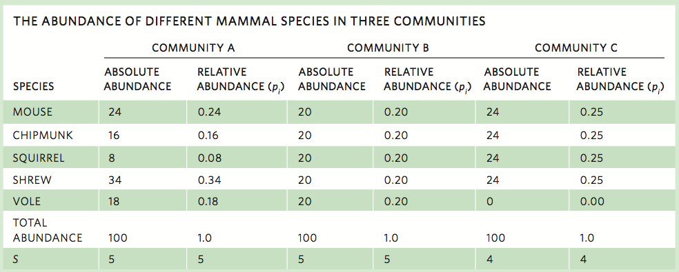
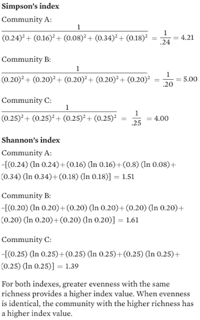
Ecologists agree that communities with more species and greater evenness have higher species diversity. Although rank abundance curves are a helpful way to visualize differences in richness and evenness among communities, they do not provide a specific value for the species diversity within a community. To quantify the species diversity of a community, we need a method of calculating a single value for species diversity. Over the years, numerous indices of species diversity have been created. We will consider the two that are most common and equally valid: Simpson’s index and Shannon’s index. Both indices incorporate species richness, which we abbreviate as S, and evenness. However, they do so in different ways.
To see how we calculate species diversity with either index, we can begin with data from three communities for which we have the absolute abundance for each of the species. From these data we can then calculate relative abundance for each of the five species in the community, which is denoted as pi. With these relative abundance data, we can calculate both Simpson’s index and Shannon’s index.
423
Simpson’s index, a measurement of species diversity, is given by the following formula:
Simpson’s index A measurement of species diversity, given by the following formula:

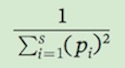
In words, this formula means that we square each of the relative abundance values, sum these squared values, and then take the inverse of this sum. For example, for Community A, Simpson’s index of species diversity is
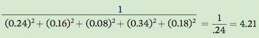
Simpson’s index can range from a minimum value of 1, which occurs when a community only contains one species, to a maximum value equal to the number of species in the community. This maximum value only occurs when all the species in the community have equal abundances.
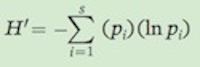
Shannon’s index (H'), also known as the Shannon-Wiener index, is another measurement of species diversity given by the following formula:
Shannon’s index (H′) A measurement of species diversity, given by the following formula:
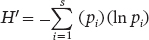
Also known as Shannon-Wiener index.
In words, this formula means that we multiply each of the relative abundance values by the natural log of the relative abundance values, sum these products, and then take the negative of this sum. For example, in Community A, Shannon’s index is
−[(0.24) (ln 0.24) + (0.16) (ln 0.16) + (0.08) (ln 0.08) + (0.34) (ln 0.34) + (0.18) (ln 0.18)]
−[(−0.34) + (−0.29) + (−0.20) + (−0.37) + (−0.31)] = 1.51
Shannon’s index can range from a minimum value of 0, which represents a community that contains only one species, to a maximum value that is the natural log of the number of species in the community. As we saw with Simpson’s index, the maximum species diversity value occurs when all species in the community have the same relative abundances.
424
Resources
The number of species in a community can be affected by the amount of available resources. Researchers have examined the effects of resources on species diversity by determining correlations between productivity and species richness in nature. They have also looked at how species richness changes when the productivity of a community is experimentally manipulated.
Natural Patterns of Productivity and Species Richness
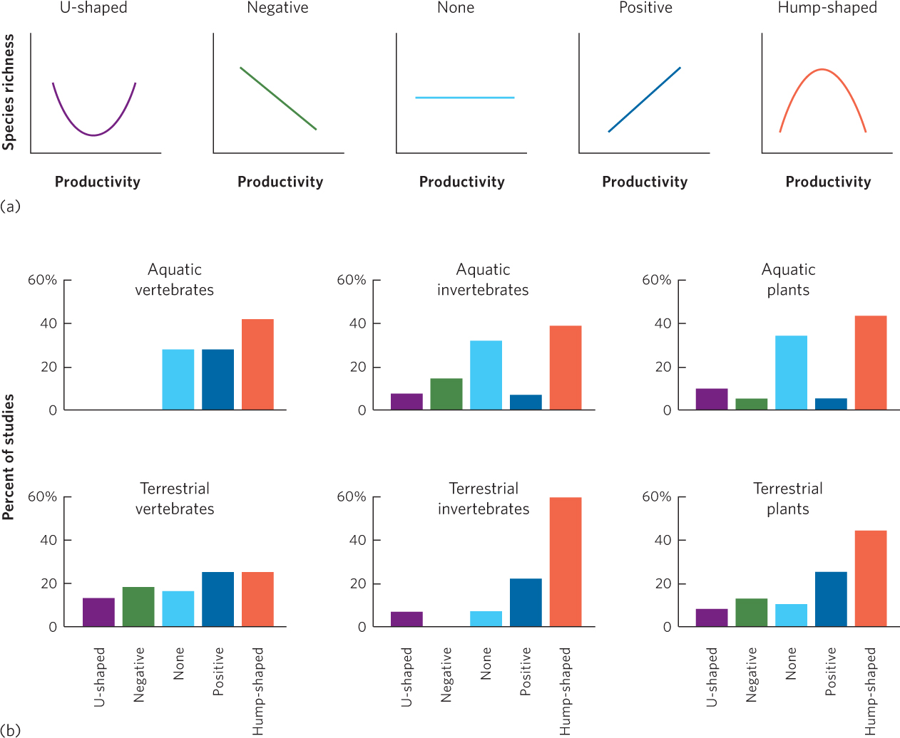
For decades ecologists have examined how the amount of biological productivity correlates with the number of species in communities. To do this they commonly measure productivity in terms of the biomass of producers or consumers that is generated over time. Among hundreds of studies that have been conducted on animals and plants in both aquatic and terrestrial environments, researchers have found a wide range of patterns, as illustrated in Figure 18.10a. In rare cases, researchers have observed a U-shaped curve in which increased productivity is associated with an initial decrease in species richness that is followed by an increase in species richness. In some studies, conducted in different biomes and in different parts of the world, diversity decreases with increasing productivity. In other cases, the correlation is positive; increases in productivity are associated with increases in species richness. In still other studies, there is no relationship between productivity and species richness. Finally, in some studies, the relationship is best described by a hump-shaped curve; initial increases in productivity are associated with an increase in species richness but further increases in productivity are associated with a decrease in species richness.
425
To gain a better sense of the relationship between productivity and species richness, a group of researchers compiled data from the hundreds of studies that have been conducted to determine the most common type of correlations. You can view their results in Figure 18.10b. Among studies of vertebrates, a hump-shaped curve was the most commonly observed relationship in aquatic systems, although hump-shaped and positive relationships were observed with similar frequency in terrestrial systems. For aquatic and terrestrial invertebrates and plants, the most commonly observed relationship was a hump-shaped curve. In short, although a variety of relationships have been observed in individual studies, the most common relationship across all studies is a hump-shaped curve. This means that a site with medium productivity has a higher species richness than sites with either low or high productivity.
Manipulations of Productivity and Species Richness
Since most communities exhibit a hump-shaped relationship between productivity and species richness, we ought to be able to predict how species richness will be affected if communities experience increased productivity. Numerous experiments have been conducted in communities of plants in which productivity has been manipulated by adding soil nutrients such as nitrogen and phosphorus. A common observation in such experiments is that species diversity declines over time. In a classic study that took place in England, known as the Park Grass experiment, researchers in 1856 began adding different types of fertilizers to several plots of grass each year while leaving other plots as unfertilized controls (Figure 18.11a). Within 2 years of starting the experiment, species richness in the fertilized plots began to decline. This decline continued for several decades and researchers determined that the amount of decline was related to the number of different nutrients that were added, as shown in Figure 18.11b. The annual addition of nutrients continues today, over 150 years later, which makes the Park Grass experiment one of the longest running experiments in the world. Although the original experiment contained treatments that were not replicated, subsequent experiments with replicated treatments have supported the conclusions of the Park Grass experiment.
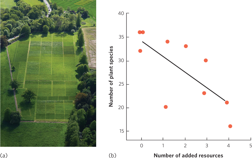
426
The Park Grass experiment and others like it have demonstrated that added fertility commonly causes a decline in the species richness of producers such as plants and algae. Typically, the total biomass of producers increases when a fertilizer is added, but this added fertilizer causes a few species to dominate the community while rare species—which are often competitively inferior—begin to decline until they eventually disappear from the community. This observation has important global ramifications because humans continue to add nutrients inadvertently to aquatic and terrestrial communities through fertilizer runoff and air pollution.
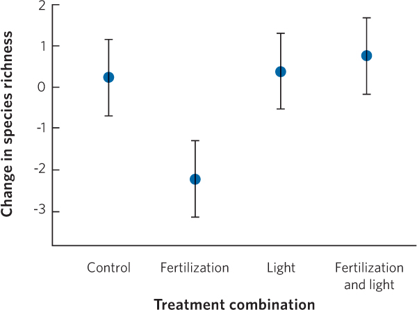
Although we know that species richness declines with increased habitat fertility, the reasons have been unclear. In the case of plant communities, ecologists have hypothesized that the increase in nutrients caused competitively dominant plants to cast more shade on the competitively inferior plants. In 2009, researchers reported the results of an experiment with four manipulations, as shown in Figure 18.12: a control community, a community that received added nutrients, a community that received added light in the plant understory, and a community that received added nutrients and added light in the plant understory. Researchers found that while adding nutrients alone caused a decline in species richness, as expected from past experiments, adding light alone had no effect. However, adding both nutrients to the soils and light to the understory reversed the decline in species richness that was seen with the addition of nutrients alone. These results confirm that soil fertility drives down species richness because it promotes growth of taller, competitively superior plants that cast shade over less-competitive plants.
Habitat Diversity
The number of species in a community can also be affected by the diversity of the habitat. Because different habitats provide places to feed and breed for different species, it seems reasonable that communities with a higher diversity of habitats— which should offer more potential niches—will also have a higher diversity of species.
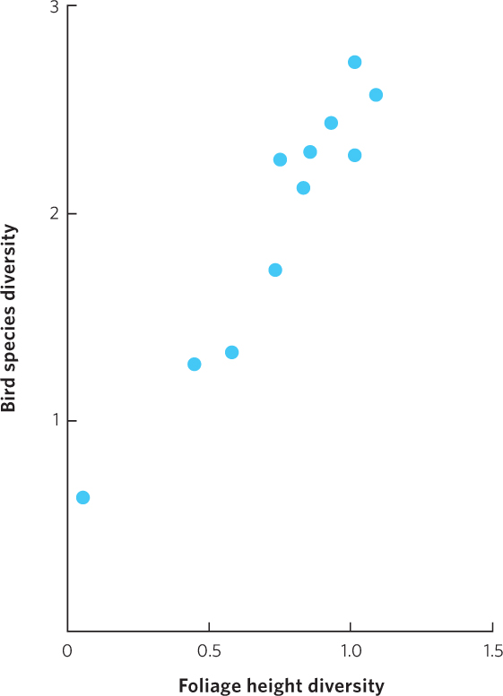
In a classic study examining the role of habitat diversity, Robert and John MacArthur investigated whether there was a relationship between the diversity of habitats among different regions of the United States and Panama and the diversity of birds in each location. To accomplish this, they measured the density of foliage at different heights above the ground in these different regions, from 0.2 to 18.3 m, and calculated the diversity of foliage heights using the Shannon index. Then they surveyed the number of breeding bird species in each area and calculated the diversity of birds, again using the Shannon index. When they graphed the relationship between the two sets of data, as shown in Figure 18.13, they found that habitats with greater foliage height diversity supported higher diversity of bird species.
Keystone Species
Keystone species A species that substantially affects the structure of communities despite the fact that individuals of that species might not be particularly numerous.
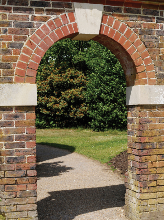
All species play a role in a community, but some species, known as keystone species, substantially affect the structure of communities despite the fact that individuals of that species may not be particularly numerous. The concept of the keystone species is a metaphor that comes from the field of architecture. In arches that are built of stone, the center stone is known as the keystone (Figure 18.14). The keystone does not carry much of the arch’s mass, but without the keystone the arch would collapse. Similarly, removing a keystone species can cause a community to collapse.
427
Keystone species affect communities in a wide variety of ways, some in their roles as predators, parasites, herbivores, or competitors. We saw an example of herbivores acting as a keystone species in Chapter 16 when we discussed an experiment in which researchers sprayed several field plots with an insecticide and left other plots unsprayed (see Figure 16.13). In the unsprayed plots, beetles consumed the competitively superior goldenrod and the competitively inferior plants survived and grew better. In the sprayed plots, the beetles remained rare and this allowed the goldenrod plants to dominate the community. In this community, the beetle was a keystone species because its presence completely altered the structure of the field community.
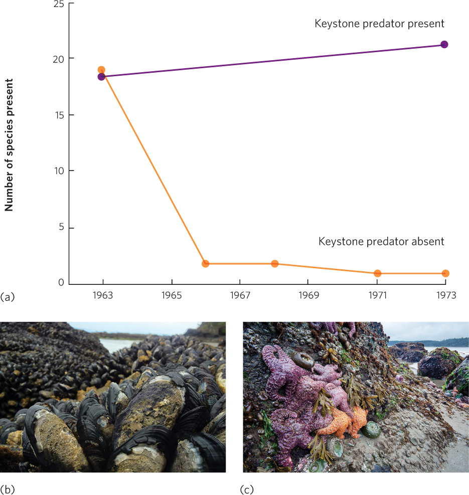
A similar scenario can be seen in the intertidal communities along the coast of Washington State. In a classic experiment, Robert Paine built cages in the intertidal zone to exclude predatory sea stars (Pisaster ochraceus) from feeding on a variety of herbivores, including mussels, barnacles, limpets, and snails. Adjacent plots of similar size were left as uncaged controls. As you can see from Paine’s data in Figure 18.15a, the control plots experienced little change in species composition from 1963 to 1973. In the caged plots, however, nearly 20 species declined to the point that they were eventually eliminated from the area. In their place, a single species of mussel (Mytilus californianus) came to dominate the rock surface. Because the mussels are the superior competitors for space on the rocks, mussels dominate the community when sea stars are absent (Figure 18.15b). When the sea stars are present, they consume large numbers of mussels, and this creates open areas of rock that many species of inferior competitors can colonize (Figure 18.15c). In short, the sea star is a keystone species in the intertidal community.
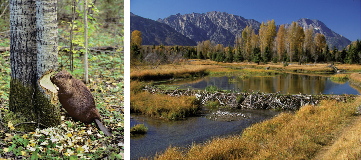
Keystone species can also affect communities by influencing the structure of a habitat. In such cases, keystone species are sometimes called ecosystem engineers. We saw an example of this with the social spiders discussed at the beginning of this chapter. One of the best-known ecosystem engineers is the beaver. Beavers build dams in streams that block the flow of water and cause large ponds to develop (Figure 18.16). Because the flowing stream is converted into a nonflowing pond, a different community of plants and animals colonize and persist in beaver ponds than in streams. Similarly, alligators create numerous large depressions in wetlands, known as gator holes, that many other species use, including fish, insects, crustaceans, birds, and mammals. Although alligators and beavers are not particularly numerous, each of these species has a major effect on its community, which makes it a keystone species.
428
Disturbances
Intermediate disturbance hypothesis The hypothesis that more species are present in a community that occasionally experiences disturbances than in a community that experiences frequent or rare disturbances.
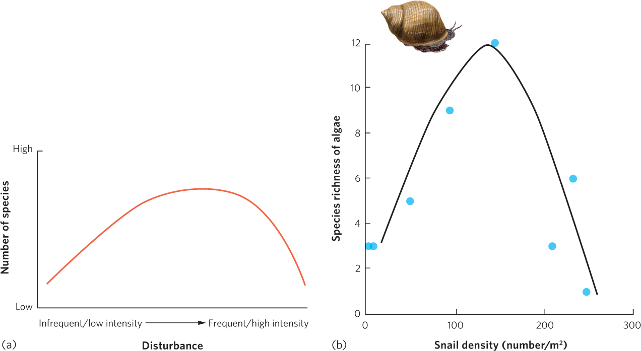
As we discussed in previous chapters, some species are well adapted to environments that experience frequent and large disturbances, such as hurricanes, fires, or intense herbivory. When environments are rarely disturbed or the disturbances have a low intensity, populations can continue to grow, resources become less abundant, and the ability to compete becomes more important for the persistence of a species. Conversely, frequently disturbed habitats typically support species that are adapted to disturbances. However, when habitats experience disturbances at some intermediate frequency, both types of species can persist and the total number of species can be higher than it would be at either extreme. The intermediate disturbance hypothesis tells us that more species are present in a community that occasionally experiences disturbances than in a community that experiences frequent or rare disturbances. As depicted in Figure 18.17a, when disturbances in a community are of low frequency or intensity, species richness is relatively low. However, when disturbances are moderate in frequency or intensity, species richness is relatively high. When disturbances are high in frequency or intensity, species richness declines.
429
The intermediate disturbance hypothesis has been observed in many different communities. One classic study was conducted by Jane Lubchenco, who manipulated the density of herbivorous periwinkle snails in tidal pools to determine how an increase in the magnitude of an herbivory disturbance would affect the species richness of algae in the pools. Her data, shown in Figure 18.17b, revealed a low richness of algal species at low snail densities, a high richness of algal species at moderate snail densities, and a low richness of algal species at high snail densities. Many similar types of studies have been conducted over several decades and a 2012 analysis of these studies found strong support for the intermediate disturbance hypothesis with respect to species richness.
430