Human activities are causing the loss of biodiversity
The current rapid decline in biodiversity is caused by the rapid increase in human populations and our many activities. Throughout this book we have mentioned how humans have altered the environment and how this has affected populations, communities, and ecosystems. Virtually all areas within temperate latitudes that are suitable for agriculture have been plowed or fenced, 35 percent of the land area is used for crops or permanent pastures, and countless additional hectares are grazed by livestock. Tropical forests are being logged at a rate of 10 million ha each year. Semiarid subtropical regions, particularly in sub-Saharan Africa, have been turned into deserts by overgrazing and harvesting firewood. Rivers and lakes are badly contaminated in many parts of the world. Gases from chemical industries and the burning of fossil fuels pollute our atmosphere. In this section, we take a global view of human impacts including habitat loss, overharvesting, introduced species, pollution, and global climate change. While each of these factors is important, keep in mind that many of these factors occur simultaneously.
Habitat Loss
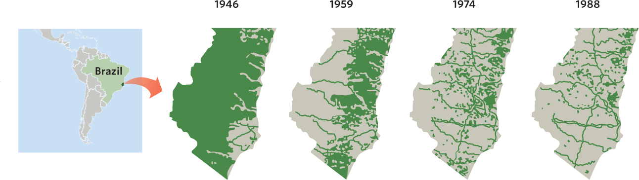
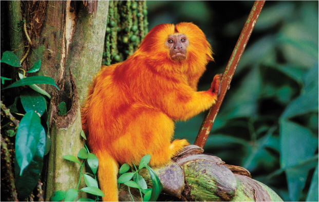
The destruction and degradation of habitat has been the largest cause of declining biodiversity. In the United States, for example, most old-growth forests were cut down in the 18th century and only a fraction of the original forest remains today. Of course, many of these forests have regrown. Logging of these new forests has typically continued using sustainable practices, although these younger forests do not provide habitat to all of the same species as the original old-growth forests did. Today, many areas of the tropics are experiencing a similar pattern of deforestation. For instance, the Atlantic forest along the coast of Brazil has been cleared so much in the past 70 years that only a small fraction of the original forest remains, as you can see in Figure 23.10. This deforestation has critically endangered many endemic birds and mammals, such as the golden lion tamarin (Leontopithecus rosalia), which lives in one tiny area of Brazil (Figure 23.11). Because such endemic species live nowhere else in the world, intense conservation efforts have focused on saving them from extinction by protecting what little habitat remains.
551
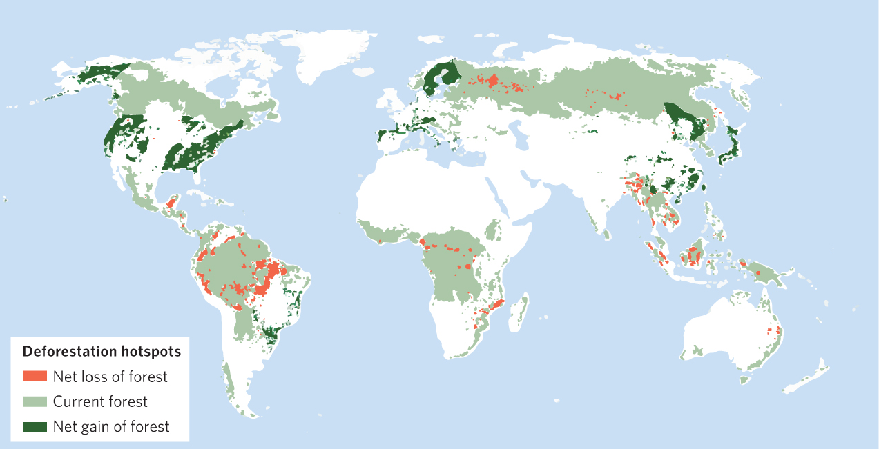
To gain insight into the global scale of habitat change, researchers have assessed how forests have been changing in more modern times. From 1980 to 2000, continued loss of forests has occurred in many regions including the Amazon, Russia, and Southeast Asia. However, there has been an increase in forests in the United States, Europe, and Northeast Asia. You can view a map of these changes in Figure 23.12. The species composition that currently exists in regions that have experienced an increase in forest cover, however, is often quite different from what existed originally, particularly in cases when a single species of tree is planted due to its high commercial value.
As we have discussed in previous chapters, habitat loss also leads to smaller habitat sizes and increased habitat fragmentation. In Chapter 22 we saw that a reduction in habitat size can lead to reduced population sizes and make it more likely a population will go extinct. This process is thought to be a significant reason that many national parks have lost species of mammals over the past 50 years, despite being protected from most harmful human activities. In addition, fragmented habitats have a high proportion of edge habitat that can alter the abiotic conditions of the interior habitat and favor edge species. We saw an example of this in Chapter 22, when we discussed the nest parasite known as the bronzed cowbird, an edge specialist that parasitizes the nests of other songbirds and leads to their decline.
Forests are not the only habitats that have been changing as a result of human activities. For example, according to the National Park Service, the original tallgrass prairie once covered 69 million ha across the middle of North America. Less than 4 percent remains today. Because the remaining areas are small fragments, many local populations of prairie plants and animals have gone extinct. A similar story exists for wetland habitats. Scientists estimate that in the 1600s, wetlands covered more than 89 million ha in the lower 48 states, but drainage for agriculture and other uses has reduced the area of wetlands by more than half. In some places such as California, 90 percent of the original wetlands have been lost. As we have seen, these habitat losses have a large negative effect on the world’s biodiversity.
552
Overharvesting
Human advances in techniques for logging trees, plowing grasslands, and capturing animals more efficiently has allowed us to harvest species at rapid rates and drive some species to extinction. For instance, during the past 3 centuries, commercial hunters in North America have hunted to extinction the Steller’s sea cow (Hydrodamalis gigas), great auk (Pinguinus impennis), passenger pigeon (Ectopistes migratorius), and Labrador duck (Camptorhynchus labradorius). Each of these once-abundant species was valued for food or feathers and they were easily killed.
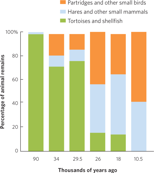
Extinction caused by overhunting and overfishing is not a recent phenomenon. Wherever humans have colonized new regions, some elements of the fauna have suffered. For example, researchers examined the skeletal remains of animals in archaeological sites around the Mediterranean region to see how human diets changed over thousands of years. At a site in current-day Italy, they found that early human populations initially ate large quantities of tortoises and shellfish, which were easy to catch. As you can see in Figure 23.13, as supplies of those foods were depleted over time, people switched to hunting hares, partridges, and other small mammals and birds.
Similar scenarios occurred when humans colonized other parts of the world. When Australia was colonized 50,000 years ago, several species of large mammals, flightless birds, and a species of tortoise soon disappeared. On Madagascar, a large island off the southeastern coast of Africa, the arrival of humans about 1,500 years ago caused the demise of 14 species of lemurs and between 6 to 12 species of elephant birds—giant flightless birds found only on that island. At about the same time, a small population of fewer than 1,000 Polynesian colonists in New Zealand hunted 11 species of moas—another group of large flightless birds—so that these birds went extinct in less than a century. In each of these cases, humans encountered island species that were unaccustomed to predation pressure. Failure to recognize danger and a lack of defenses made these species particularly vulnerable to human hunting.
Overharvesting of species continues in modern times. In some cases, the harvesting is part of an illegal trade in plants and animals, an endeavor that is valued at $5 billion to $20 billion annually. For example, many animal skins are sold for furs and some cultures believe that certain animal body parts have medicinal value. Some species of rare trees, such as big-leaf mahogany (Swietenia macrophylla), are sold for their lumber, while species of rare flowers, such as endangered species of orchids, are sold for their beauty.
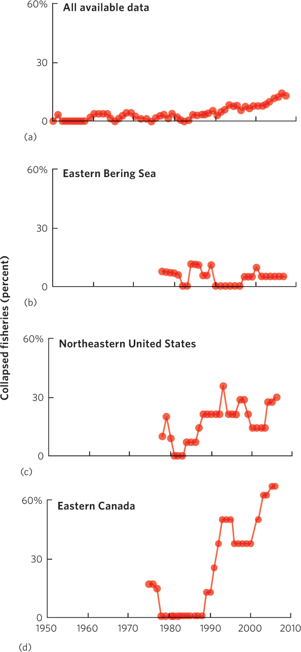
Governments frequently regulate the harvest of plants and animals in the wild to ensure that the harvested species will persist for future generations to enjoy. However, harvesting regulations must balance not only the good of the harvested population but also the human employment that the harvest supports. As a result, some regulations set harvest levels that do not stop populations from declining. In marine environments, for example, modern fishing techniques have made it much easier to harvest enormous numbers of fish and shellfish. These techniques include fishing lines that are several kilometers long with thousands of baited hooks, nets that can surround schools of fish up to 2 km in diameter and 250 m deep, and huge trawlers that can scrape large areas of the ocean bottom. The ability to fish more efficiently and to cover larger areas has caused a decline of many fish populations around the world. When a fishery no longer has a population that can be fished, it is called a collapsed fishery. A recent analysis of commercially captured fish and other seafood found that since the 1950s there has been a steady increase in the percent of collapsed fisheries. Some of the most complete data exists for fish and shellfish in North America. As you can see in Figure 23.14, the percentage of collapsed fisheries increased to 14 percent by 2007. Some regions, such as the eastern Bering Sea off the shores of Alaska, have very few collapsed fisheries. In contrast, collapsed fisheries occur in more than 25 percent of species assessed off the coast of the northeastern United States and more than 60 percent of species assessed off the coast of eastern Canada.
553
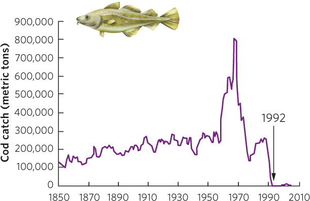
For example, consider the case of the Atlantic cod, a species of fish caught by commercial trawlers. On the Grand Banks fishery off the coast of Newfoundland in Canada, the amount of cod caught from 1850 to 1960 slowly increased from 100,000 to 300,000 metric tons, as shown in Figure 23.15. During the 1970s and 1980s, new technologies—including advanced sonar, GPS, and larger trawlers—allowed a large increase in the number of cod caught, with a peak catch of 800,000 metric tons. However, the population crashed to very low levels in the early 1990s, leading the Canadian government to close the fishery in 1992. In 2012, 20 years after the ban was imposed, scientists reported that there were finally signs that the cod population was beginning to rebound.
554
The decline in cod also occurred in New England. Because it was not as severe as the decline off the Newfoundland coast, fishing continued although the quota of cod that could be caught was reduced. By 2010, the U.S. government greatly reduced the amount of cod that could be caught by commercial anglers, in the hope that the population would rebound. An assessment in 2011 found that the cod population had been very slow to respond, and so limits were reduced even further for 2013 through 2016. U.S. cod fishermen lobbied for higher cod quotas so that they could continue to make a living. However, the government biologists argued that if the cod limits were not lowered substantially, there would soon be no cod left to catch. This debate mirrored the Canadian experience of two decades earlier. At that time, despite low cod numbers, the Canadian government was under pressure from cod fishermen to allow continued fishing. The government agreed, but soon the number of fish fell so much that cod fishing had to be completely stopped and 35,000 Canadian fishermen lost their livelihood. Although reducing the harvest of overharvested species has real economic impacts on those employed in the industry, failure to restrict the harvest hastens the decline of the species to levels at which there are no individuals left to harvest.
Introduced Species
Another cause of declines in biodiversity is the increasing number of species that are introduced from one region to another. Some of these introductions are intentional, such as when tropical plants are sold for houseplants in temperate parts of the world. Often, however, species are introduced by accident, as we saw in Chapter 15 with the many pathogens that have moved between continents and have caused emerging infectious diseases. Although only about 5 percent of introduced species become established in a new region, those that do can have a variety of effects. Some introduced species provide important benefits, such as the common honeybee that was introduced to North America from Europe in the 1600s. Other introduced species can have substantial negative effects on native species, like the brown tree snake introduced to the island of Guam, which we discussed in Chapter 14 (see Figure 14.2). In that case, the snake caused the decline or extinction of nine species of birds, three species of bats, and several species of lizards. In general, introduced species that compete with native species rarely cause extinction of native species whereas introduced species that act as predators or pathogens on native species can cause large population declines and extinctions of native species.
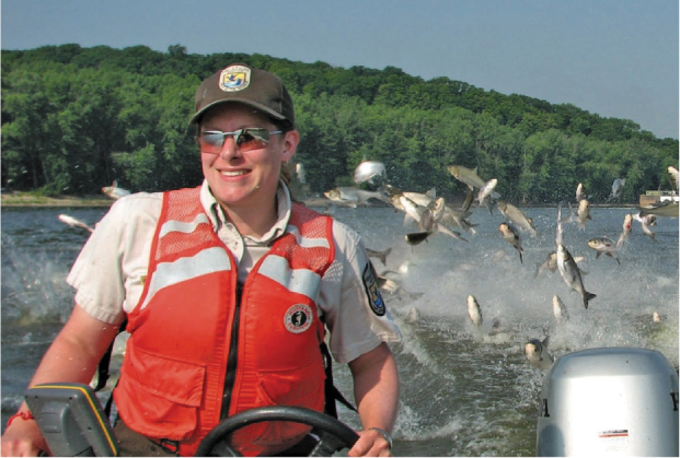
One of the highest-profile introduced species today is the silver carp (Hypophthalmichthys molitrix), a species of fish that has been introduced around the world because it consumes excess algae in water treatment plants and aquaculture operations. Brought to the United States in the 1970s, the carp escaped captivity in the 1980s when floodwaters washed them out of ponds and into the Mississippi River. The species rapidly spread through the Mississippi River and its tributaries, including the Illinois River. The primary concern is that the Illinois River connects the Mississippi River to Lake Michigan and, thus, the carp has the potential to invade the entire Great Lakes ecosystem. In 2010, the carp’s DNA was detected in Lake Michigan, which suggests that the carp may be spreading throughout the Great Lakes. The silver carp is such a voracious consumer of algae that scientists worry it will compete with native consumers of algae, which serve as a key link in the food chain for many species of commercially important fish. The carp also has the unusual behavior of jumping out of the water when a boat passes by. Since the silver carp can reach a mass of 18 kg and jump up to 3 m out of the water, it poses a serious safety risk to boaters (Figure 23.16). It will take researchers several years before they can assess the full impact of the silver carp on North American waters.
555
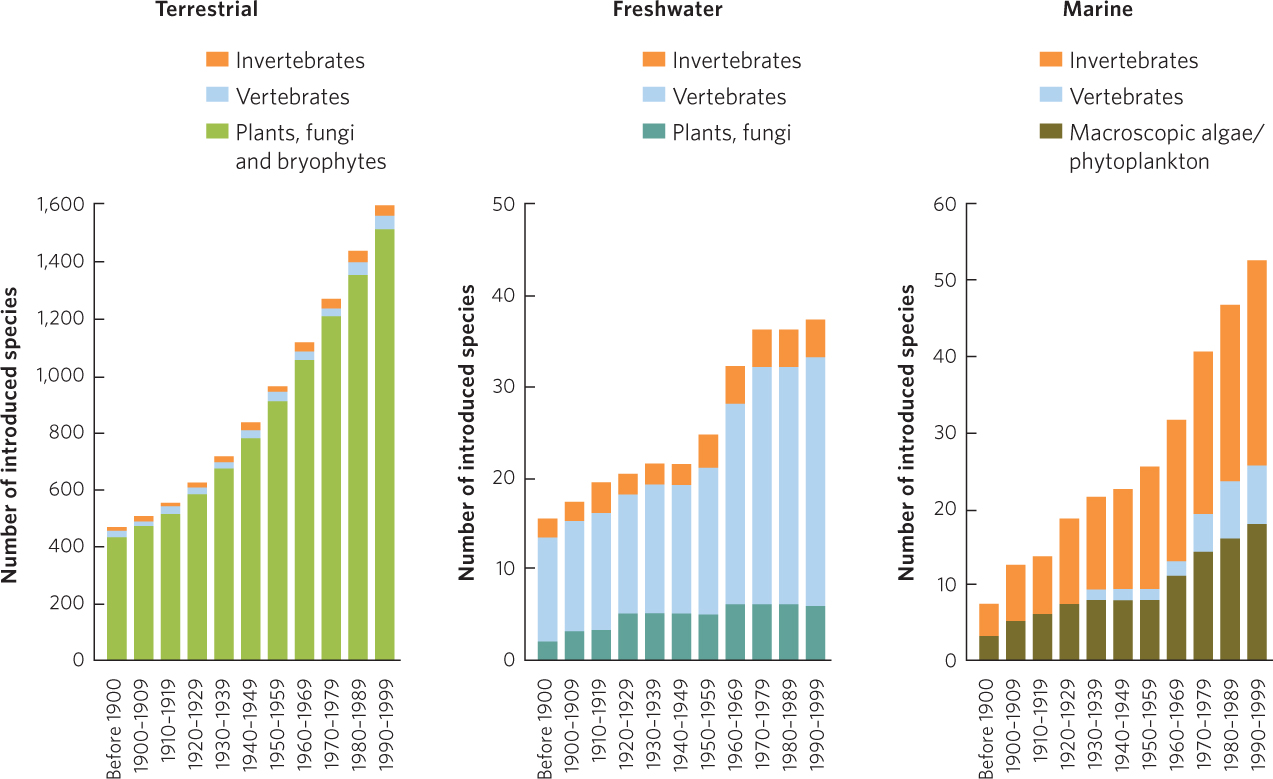
Some of the most complete data on introduced species exist for the Nordic countries of Sweden, Finland, Norway, Denmark, and Iceland. As you can see in Figure 23.17, the number of introduced species in this area has rapidly increased since 1900. Across terrestrial, freshwater, and marine ecosystems, there are currently more than 1,600 introduced species in the Nordic region. Similarly, during the past 200 years in North America thousands of species have been introduced, many of which have spread rapidly and are considered invasive species. According to the Center for Invasive Species and Ecosystem Health, North America currently has a large number of invasive species that include nearly 200 pathogens, 300 vertebrates, 500 insects, and 1,600 plants. One introduced species with largely unappreciated negative effects is the domestic house cat. In 2013, researchers examined predation by free-ranging domestic cats in the United States and found that the cats killed 1.4 to 3.7 billion birds and 7 to 21 billion mammals each year. Collectively, these data suggest that introduced species have the potential to cause widespread effects on native species and ecosystems. As the movement of people, cargo, and species becomes more common among the regions of the world, the unique species compositions originally found in different regions are slowly become more similar, a process known as biotic homogenization.
Biotic homogenization The process by which unique species compositions originally found in different regions slowly become more similar due to the movement of people, cargo, and species.
556
Pollution
We have talked about many types of pollution throughout this book. For example, in Chapter 2 we discussed acid precipitation and in Chapter 21 we looked at the effects of adding excess nutrients to bodies of water. Both examples demonstrated the harmful effects of pollutants on biodiversity.
The group of chemicals collectively called pesticides is a common type of pollutant. Pesticides include insecticides that kill insects, herbicides that kill plants, and fungicides that kill fungi. These chemicals are designed to target a particular type of pest; ideally they will not harm nonpests in the ecosystem. However, some pesticides do kill nonpests, either directly, by being toxic, or indirectly, by altering food webs, as we saw in the wetland study discussed at the end of Chapter 18. In that study, a very small amount of an insecticide, while not directly toxic to tadpoles, was toxic to zooplankton. The death of zooplankton set off a chain of events in the food web that prevented the tadpoles from obtaining enough food to metamorphose before the pond dried. By indirect effect, the insecticide caused the death of approximately half of the tadpoles.
A classic study on pesticides examined the role of the insecticide DDT on birds of prey. During the 1950s and 1960s in the United States, populations of many predatory birds, particularly the peregrine falcon (Falco peregrinus), bald eagle, osprey (Pandion haliaetus), and brown pelican (Pelecanus occidentalis), declined drastically. Several of these species disappeared from large areas and the peregrine falcon disappeared from the entire eastern United States. The causes of these population declines were traced to pollution of aquatic habitats by DDT, a pesticide that was widely used to control crop pests and mosquito vectors of malaria after World War II.
When this pesticide enters a water body, it binds to particles, including algae, to become about 10 times more concentrated than it was in the water. When the algae are consumed by zooplankton, DDT accumulates in fat tissues until the zooplankton have a concentration that is about 800 times higher than in the water, as shown in Figure 23.18. The process of increasing the concentration of a contaminant as it moves up the food chain is known as biomagnification. When small fish eat the zooplankton and large fish eat the small fish, DDT can be further concentrated about 30-fold. Finally, when a fish-eating bird such as an osprey consumes a large fish, DDT becomes concentrated another 10-fold. In short, at the top of the food chain the insecticide is 276,000 times more concentrated in the body of the fish-eating bird than it was in the water. Such a high concentration in predatory birds interferes with their physiology in a way that causes the eggs they lay to have very thin shells. When the parents sit on these thin-shelled eggs, the egg shells break, and the embryos die. This eggshell thinning caused the populations of predatory birds to plummet during the 1960s.
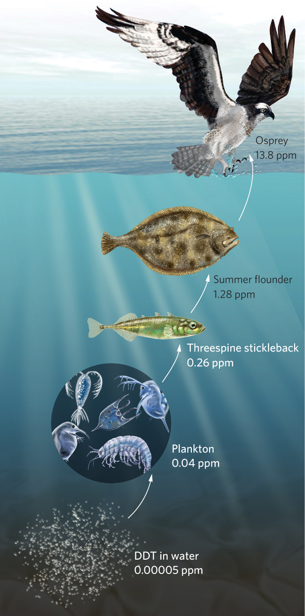
Biomagnification The process by which the concentration of a contaminant increases as it moves up the food chain.
557
ANALYZING ECOLOGY
Contaminant Half-Lives
Half-life The time required for a chemical to break down to half of its original concentration.
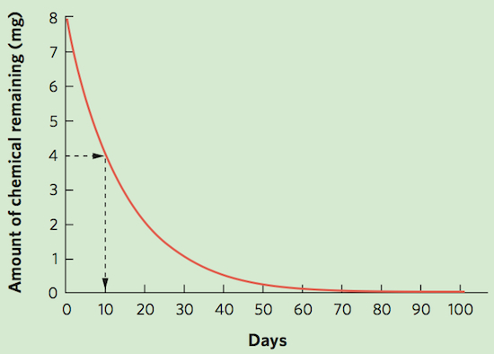
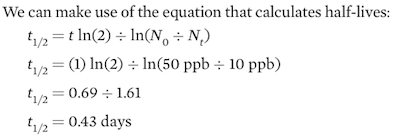
As we have mentioned, an important factor in determining whether a contaminant such as a pesticide or radioactive compound affects the environment is the length of time the chemical persists in the environment. A helpful way to assess this persistence is to measure the time required for the chemical to break down to half of its original concentration, which we call the half-life. To calculate the half-life, we start by recognizing that most chemicals have a breakdown rate that follows a negative exponential curve, as shown in the accompanying figure for a hypothetical chemical. If we were to start with 8 mg of the chemical and want to ask how many days it takes until the chemical breaks down to only 4 mg, we see that it takes 10 days. To break down by half again, from 4 to 2 mg, it takes another 10 days.
It is relatively easy to determine the half-life when we have a line graph. However, it is more difficult when we only have two data points: the amount of a chemical we start with and the amount of chemical remaining at some later point in time. In such cases, we can make use of an equation that calculates half-lives:
t1/2 = t ln(2) ÷ ln(N0 ÷ Nt)
where t1/2 is the half-life of the chemical, N0 is the initial amount of the chemical, and Nt is the amount of chemical after some amount of time (t) has elapsed. For example, using data from the figure, we begin with 8 mg of a chemical and after 30 days we have 1 mg remaining. Using these data, we can calculate a half-life:
t1/2 = 30 ln(2) ÷ ln(8 ÷ 1)
t1/2 = 20.8 ÷ 2.08
t1/2 = 10 days
Note that this is the same answer we obtained by estimating the half-life directly from the curve.
Understanding the connection between DDT and declining bird populations led the United States government to ban the use of DDT and related pesticides in 1972. Alternative insecticides have since been developed. With the help of many biologists who hand-reared hundreds of predatory birds, populations of species such as the peregrine falcon and bald eagle have rebounded. DDT is still used in many tropical countries, although now in a limited manner, such as in houses to control the mosquitoes that carry malaria.
Global Climate Change
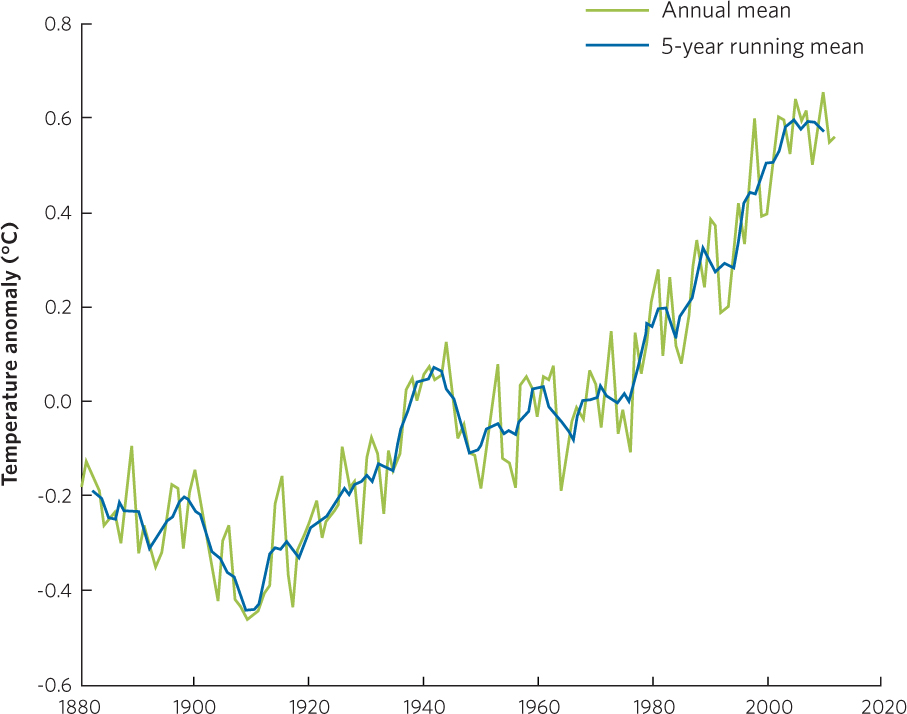
Changing global climates play both future and current roles in the biodiversity of species. In Chapter 5 we discussed the greenhouse effect and how gases such as water vapor, CO2, methane, and nitrous oxide allow our planet to be warmed naturally by absorbing infrared radiation emitted by Earth and then reradiating a portion back toward Earth. During the past century, human activities have increased the concentration of these greenhouse gases in the atmosphere (see “Ecology Today” in Chapter 4), as well as the gases used as refrigerants known as chlorofluorocarbons (CFCs). One result of the increase in greenhouse gases has been an increase in the average temperature on Earth. From 1880, when the earliest measurements were taken, to 2013, the temperature on Earth has increased an average of 0.8°C, as illustrated in Figure 23.19. While this is an average, some parts of the world such as northern Canada and Alaska have experienced temperature increases as high as 4°C.
558
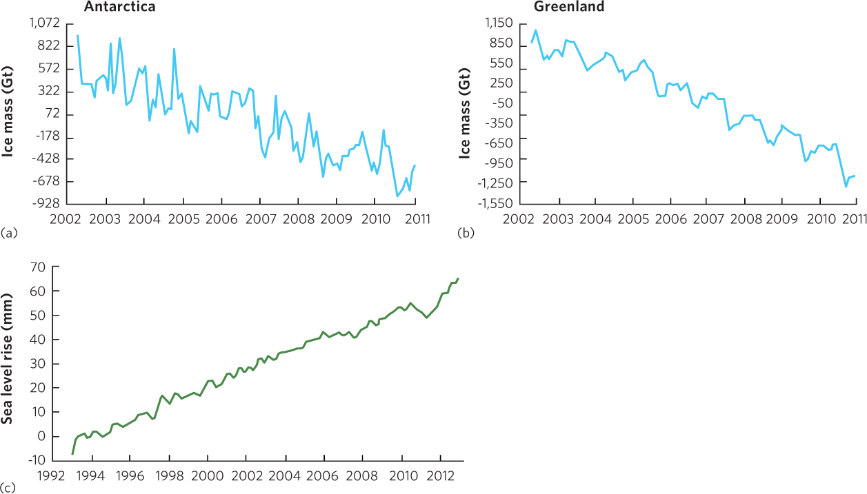
Global warming has caused a number of effects that can be readily observed. For example, we might expect warmer temperatures to cause more of the world’s ice to melt. As we noted at the end of Chapter 5, the massive polar ice cap in the Arctic has decreased in mass by 45 percent during the past 30 years. Similarly, the decline in ice from 2002 to 2010 has been more than 1,300 metric gigatons for Antarctica and more than 1,700 gigatons for Greenland. You can view these data in parts a and b of Figure 23.20. All of this melting ice, combined with an overall warming of the oceans that causes water to expand, should cause a rise in sea levels. Researchers have examined water gauges for ocean tides since 1870 and, as expected, have observed a steady increase in sea level; today the sea level is 0.2 m higher than it was in 1870. During the past 20 years, the sea level has been rising more than 3 mm per year, as shown in Figure 23.20c. At this rate, the sea will rise 0.3 m every 100 years, which is enough to dramatically affect habitats on islands and along coastlines.
559
As we have seen throughout this book, these changes in global temperatures are already affecting species. In Chapter 8 we discussed how many species of plants now flower earlier in the spring than they did in past decades and how some species of birds and amphibians now breed earlier. In Chapter 11 we saw that warming ocean temperatures have caused a major shift in the fish species that live in the North Sea. Several of the species that historically lived in the North Sea have moved farther north to cooler waters while a number of species that had lived in more southern waters moved up into the North Sea; this changed the species composition of the community.
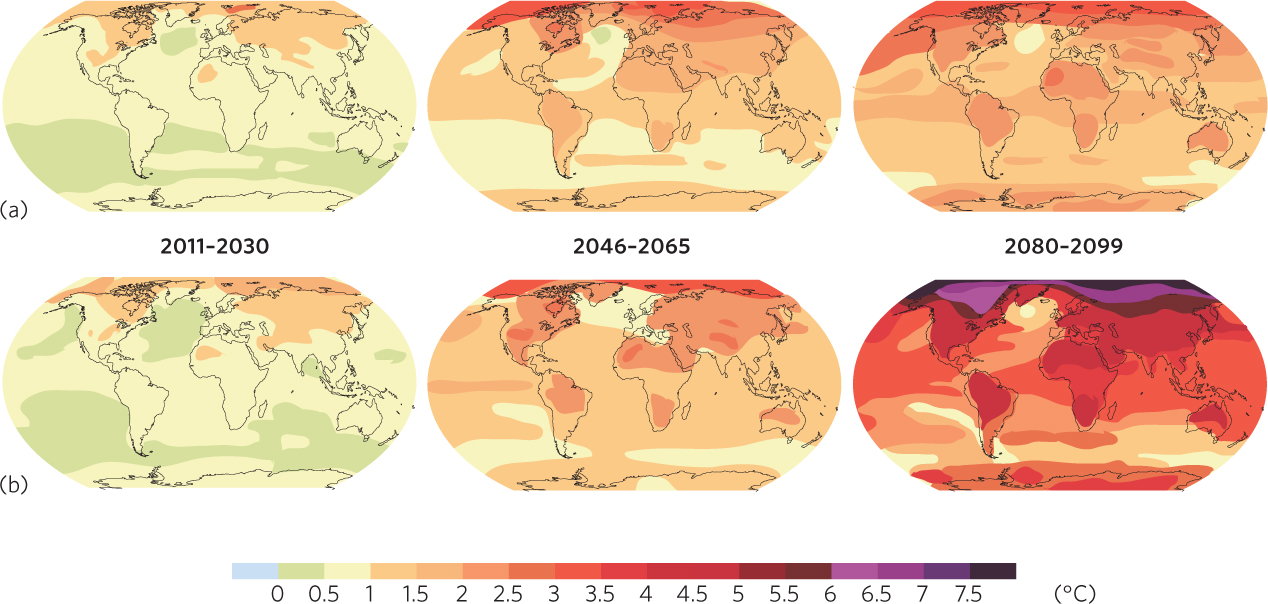
Global climate change has not yet led to the widespread extinction of species. However, it is difficult for scientists to predict what will happen to global climates in the future and how these changes might affect species and ecosystems. To accomplish this, researchers have developed computer models that make predictions about how temperature and precipitation will change over future decades. One of the critical factors is how much we continue to increase the amount of CO2 in the atmosphere. As you can see in Figure 23.21, researchers predict that a small increase in CO2 will cause the northern latitudes to experience an additional 4°C rise in average temperatures by the end of this century. A large increase in CO2 will raise temperatures by an additional 7°C. Researchers predict that these changes will cause extreme weather events such as hurricanes and droughts to occur more frequently. In addition, some regions of the world will receive more annual precipitation than is currently typical while other regions will receive less. While specific predictions vary with different models, the distributions of organisms in nature will probably shift as the Earth’s climates change over the next century.