626

Chapter 1

1.1 Population: The population is not explicitly defined. From the context of the problem, we might assume it to be all American adults. However, as a phone survey, the population might be more appropriately defined as American adults with telephones. Sample: The sample is the 1500 randomly selected American adults who were called in this research poll.

1.2 This is an observational study. The researcher examined student comments, but no treatment was applied to the students.

Chapter 2

2.1 This is not a simple random sample. Not every possible group of four students can be selected. For example, four students sitting in the same row can never be selected.

2.2 Step 1: Label. For the 20 teaching assistants (TAs), we use labels

01, 02, 03, . . . , 18, 19, 20

Specifically, the list of TAs with labels attached is

Step 2: Software or table. We used the Research Randomizer and requested that it generate one set of numbers with three numbers per set. We specified the number range as 1 to 20. We requested that each number remain unique and that the numbers be sorted least to greatest. We asked to view the outputted numbers with the markers off. After clicking the “Randomize Now!” button, we obtained the digits 1, 5, and 14. (Of course, when you use the Research Randomizer, you will very likely get a different set of three numbers.) The sample is the TAs labeled 01, 05, and 14. These are Alexander, Gogireddy, and Scarborough.

To use the table of random digits, we might enter Table A at line 116 (any line may be used), which is

14459 26056 31424 80371 65103 62253 50490 61181

The first 13 two-digit groups in this line are

14 45 92 60 56 31 42 48 03 71 65 10 36

We used only labels 01 to 20, so we ignore all other two-digit groups. The first 3 labels between 01 and 20 that we encounter in the table choose our sample. Of the first 13 labels in line 116, we ignore 10 of them because they are too high (over 20). The others are 14, 03, and 10. The sample is the TAs labeled 03, 10, and 14. These are Book, Ozanne, and Scarborough.

Chapter 3

3.1 Recall our quick method for finding the margin of error for 95% confidence:

Here with n = 1024, the margin of error is

3.2 Now, n = 4000, so the margin of error for 95% confidence is

which is smaller than for the smaller sample (n = 1024).

Chapter 4

4.1 The question is clearly slanted toward a positive (Yes) response because the question asks the respondent to consider “escalating environmental degradation and incipient resource depletion.”

4.2 Label faculty 01, 02, . . ., 18. Label students 01, 02, . . ., 80. Starting at line 111 in Table A, we choose the person labeled 12 as the faculty member and the person labeled 38 as the student. Answers will vary with technology.

627

Chapter 5

5.1

Chapter 6

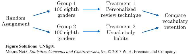
6.1 There are two explanatory variables. They are brand of dripper and wet/dry filter. The response variable is the score for flavor on a scale from 1–10. There are three brands of drippers and wet or dry filters, so there are a total of six treatments (the six brand of dripper and wet/dry filter combinations). Two cups of coffee are brewed at each of these six treatments, so 12 cups of coffee are needed. Here is a diagram describing the treatments.

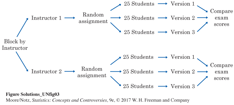
6.2 In this experiment, the instructors are the blocks, for which the 75 students in each class are split randomly into three groups of 25, each receiving a different version of the test. Exam scores would then be compared as the response variable. Here is a sample diagram.

Chapter 7

7.1 Although this study exposes the students to minimal risk, it is always a good idea to seek Institutional Review Board approval before proceeding with any study involving human subjects.

7.2 This is a complicated situation. This patient’s underlying disease appears to be impairing his decision-making capacity. If his wishes are consistent during his lucid periods, this choice may be considered his real preference and followed accordingly. However, because his decision-making capacity is questionable, family members should be contacted about the procedure. Getting a surrogate decision maker involved might help determine what his real wishes are.

628

7.3 Confidentiality. While the results are not reported to your insurance company or placed on your medical records, the company that completed the procedure and mailed your results has the ability to link you to your data.

7.4 No. Observational studies can still meet all of these requirements and be deemed “ethical.”

Chapter 8

8.1 The number of drivers is usually much greater between 5 and 6 P.M. (rush hour) than between 1 and 2 P.M. Thus, we would expect the number of accidents to be greater between 5 and 6 P.M. than between 1 and 2 P.M. It is therefore not surprising that the number of traffic accidents attributed to driver fatigue was greater between 5 and 6 P.M. than between 1 and 2 P.M. This is an example where the proportion of accidents attributed to driver fatigue is a more valid measure than the actual count of accidents.

8.2 Although In-N-Out Burger was rated first both times, there may be some reliability concerns since the same restaurant (Five Guys Burger and Fries) received drastically different ratings between 2011 (third) and 2014 (seventh).

Chapter 9

9.1 This is not plausible From the information given, we can determine how many melons are produced per square foot:

So, as stated, the field would need to produce more than 17 melons per square foot, which is quite unreasonable.

9.2 The percent increase from the first quiz to the second quiz is

However, the percent decrease from the second to the third quiz is

Chapter 10

10.1 The “state” variable is a categorical variable. For categorical variables, we should use either a bar graph or a pie chart. However, because we are not comparing parts of a whole and the percents do not add up to 100%, a bar graph is more appropriate.

10.2

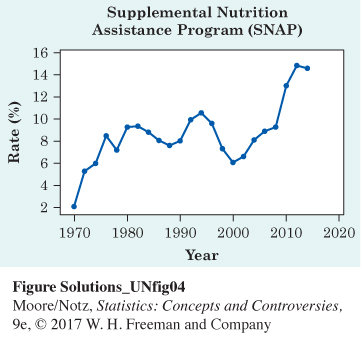
The percent of the population receiving SNAP benefits rose sharply between 1970 and 1976, then remained relatively stable (rising and falling slightly) until 1994. From 1994 to 2000, there was a sharp decline, followed by a sharp increase in participation through 2014.

Chapter 11

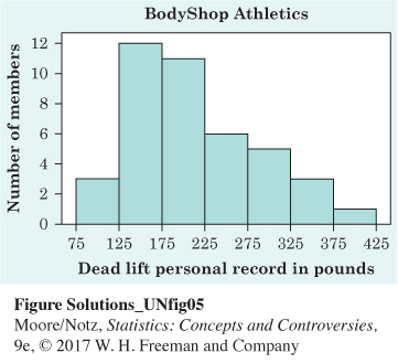
11.1 Step 1: Divide the range of the data into classes of equal width. The data in the table range from 95 to 405, so we choose as our classes

75 ≤ weight < 125

125 ≤ weight < 175

. . .

375 ≤ weight < 425

Step 2: Count the number of individuals in each class. For example, there are three members in the first class, 12 members in the second class, and so on, up to one member in the final class.

629

Step 3: Draw the histogram. Mark on the horizontal axis the scale for the variable whose distribution you are displaying. That’s “Dead Lift Personal Record in Pounds” here. The scale runs from 75 to 425 because that range spans the classes we chose. The vertical axis contains the scale of counts. Here that is “Number of Members.” Each bar represents a class. The base of the bar covers the class, and the bar height is the class count. There is no horizontal space between bars unless a class is empty, so that its bar has height zero. The following figure is our histogram.

11.2 The distribution is mostly symmetric (perhaps slightly left skewed), with a center between 65 and 67 inches. The data are spread between 57 and 73 inches, with no outliers.

Chapter 12

12.1 There are 22 observations, so the median lies halfway between the 11th and 12th numbers. The middle two values are 35 and 41, so the median is

There are 11 observations to the left of the location of the median. The first quartile is the median of these 11 numbers and so is the sixth number. That is,

Q₁ = 11

The third quartile is the median of the 11 observations to the right of the median’s location:

Q₃ = 47

12.2

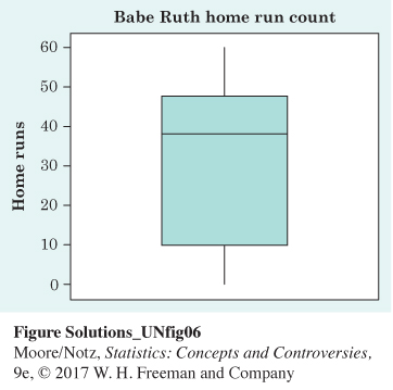
The median (38) and the third quartile (47) for Ruth are slightly larger than for Bonds and Aaron. The distribution for Ruth appears more skewed (left-skewed) than for Bonds and Aaron. If one examines Ruth’s career, one finds that he was a pitcher for his first six seasons, and during those seasons, he did not have many plate appearances. Hence, he has six seasons of very low home run counts, resulting in a left-skewed distribution.

12.3 To find the mean,

To find the standard deviation, use a table layout:

The variance is the sum divided by n − 1, which is 23 − 1, or 22.

630

The standard deviation is the square root of the variance.

The mean (32.83) is less than the median of 34. This is consistent with the fact that the distribution of Aaron’s home runs is slightly left-skewed.

Chapter 13

13.1 The central 95% of any Normal distribution lies within two standard deviations of the mean. Two standard deviations is 5 inches here, so the middle 95% of the young men’s heights is between 65 inches (that’s 70 − 5) and 75 inches (that’s 70 + 5).

13.2 The standard score of a height of 72 inches is

13.3 To fall in the top 25% of all scores requires a score at or above the 75th percentile. Look in the body of Table B for the percentile closest to 75. We see that a standard score of 0.7 is the 75.80 percentile, which is the percentile in the table closest to 75. So, we conclude that a standard score of 0.7 is approximately the 75th percentile of any Normal distribution.

To go from the standard score back to the scale of SAT scores, “undo” the standard score calculation as follows:

observation = mean + standard score × standard

deviation

= 500 + (0.7) (100) = 570

A score of 570 or higher will be in the top 25%.

For scores at or below 475:

Looking up a standard score of 20.3 in Table B, we find 38.21% of scores will be at or below 475.

For scores at or above 580:

Looking up a standard score of 0.8 in Table B, we find 78.81% of scores will be below 580. Taking the complement, 100% − 78.81%, we find that 21.19% of scores will be at or above 580.

Chapter 14

14.1 The researchers are seeking to predict IQ from brain size. Thus, brain size is the explanatory variable. The response variable is IQ. The following figure is a scatterplot of the data.

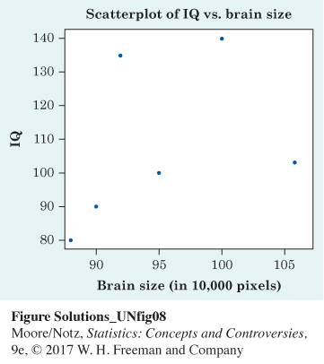
14.2 There is a weak positive association. There is no pronounced form other than evidence of a weak positive association. There are no outliers.

14.3 One might estimate the correlation to be about 0.3 or 0.4. The actual correlation is 0.38.

Chapter 15

15.1 The predicted humerus length for a fossil with a femur 70 cm long is

humerus length = −3.66 + (1.197)(70) = 80.13 cm

15.2 The proportion of the variation in hot dog prices explained by the least-squares regression of hot dog prices on beer prices (per ounce) is r² = (0.36)² = 0.1296 or 12.96%.

15.3 The observed relationship is certainly not direct causation. Some confounding is possible (food prices may be somewhat standardized at a baseball stadium), but the correlation is most likely due to common response: prices for food and beer probably depend on general economic trends.

Chapter 16

16.1 The CPI for 1984 is 103.9, and the CPI for 2015 is 238.7. So the 1984 median salary in 2015 dollars is

16.2 The CPI for 1984 is 103.9, and the CPI for 2013 is 233.0. So the 1984 earnings in 2013 dollars are

631

In terms of real earnings, the change between 1984 and 2013 is

That is, the real earnings have decreased by 18.9%.

Chapter 17

17.1. As long as the coin is fair so that heads and tails are equally likely, all three sequences of 10 particular outcomes are equally likely, even though the first one looks the most “random.” Each sequence of 10 particular outcomes has a probability of .

17.2. A correct statement might be, “If you tossed a coin a billion times, you could predict a nearly equal proportion of heads and tails.”

Chapter 18

18.1. Let a pair of numbers represent the number of spots of the up-face of the first and second die, respectively. The probability of rolling a 7 is

The probability of rolling an 11 is

By Rule D, the probability of rolling a 7 or an 11 is

18.2. 45.6% is 2 standard deviations below the mean of 50%. The 68–95–99.7 rule tells us that 5% will be more than 2 standard deviations away from the mean. Half of 5%, or 2.5%, will be more than 2 standard deviations below the mean; that is, the probability that fewer than 45.6% say Yes is 0.025.

Chapter 19

19.1. In a standard deck of cards, 13 of the cards are spades, 13 are hearts, 13 are diamonds, and 13 are clubs. We need two digits to simulate one draw:

00, 01, . . . , 12 = spades

13, 14, . . . , 25 = hearts

26, 27, . . . , 38 = diamonds

39, 40, . . . , 51 = clubs

Ignore two-digit groupings of 52, 53, . . . , 99.

19.2. Step 1. The first card selected can be either a spade, heart, diamond, or club. For each possibility for the first card, the second card can be either a spade, heart, diamond, or club, but the number of spades, hearts, diamonds, or clubs left depends on the suit of the first card selected (there are only 12 of that suit and 13 of the other suits).

Step 2. The assignment of probabilities to the first card selected: 00 to 12 = spade, 13 to 25 = heart, 26 to 38 = diamond, 39 to 51 = club. Skip any other digits. The assignment of the second card selected: If the first card selected is a spade, then use 00 to 11 = spade, 12 to 24 = heart, 25 to 37 = diamond, 38 to 50 = club. Skip any other digits. If the first card selected is a heart, then use 00 to 12 = spade, 13 to 24 = heart, 25 to 37 = diamond, 38 to 50 = club. Skip any other digits. If the first card selected is a diamond, then use 00 to 12 = spade, 13 to 25 = heart, 26 to 37 = diamond, 38 to 50 = club. Skip any other digits. If the first card selected is a club, then use 00 to 12 = spade, 13 to 25 = heart, 26 to 38 = diamond, 39 to 50 = club. Skip any other digits.

Step 3. The 10 repetitions starting at line 101 in Table A gave

Line 101: heart, heart

Line 102: club, club

Line 103: club, club

Line 104: heart, spade

Line 105: diamond, club

Line 106: club, club

Line 107: heart, spade

Line 108: spade, heart

Line 109: diamond, spade

Line 110: diamond, club

We got the same suit three out of ten times, so we estimate the probability to be 3/10.

Chapter 20

632

20.1. The expected value is (0)(0.67) + (1)(.14) + (2)(.12) + (3)(.05) + (4)(.02) = 0.61. The average number of children under 18 in a household is 0.61.

20.2. Because Stephen Curry makes about half of his field-goal shots, we would expect around two field-goal attempts to make his first field-goal shot (more precisely, shots before he makes his first).

To estimate the expected value using simulation methods, the answer will depend on the starting point in Table A and on the assignment of two-digit pairs. For example, use 00 to 48 to represent a made shot and 49 to 99 to represent a missed shot. Starting on line 115 of Table A, the number of shots until the first made shot is 2, 1, 4, 1, 1, 1, 4, 1, 1, 2. The average of these 10 outcomes is 1.8. Thus, the estimate of the expected number of shots needed to make his first field goal is 1.8 shots based on this simulation.

Chapter 21

21.1. The 95% confidence interval for the proportion of all adult Americans who believe gambling is morally wrong is

Interpret this result as follows: we got this interval by using a recipe that catches the true unknown population proportion 95% of the time. The shorthand is, we are 95% confident that the true proportion of adult Americans who believe gambling is morally wrong lies between 28.2% and 33.8%.

21.2. The 99% confidence interval for the proportion of all adult Americans who believe gambling is morally wrong is

Interpret this result as follows: we got this interval by using a recipe that catches the true unknown population proportion 99% of the time. The shorthand is, we are 99% confident that the true proportion of adult Americans who believe gambling is morally wrong lies between 27.4% and 34.6%.

21.3. The 95% confidence interval for μ uses the critical value z* = 1.96 from Table 21.1. The interval is

= 126.1 ± 1.96(1.79)

= 126.1 ± 3.5

We are 95% confident that the mean blood pressure for all executives in the company between the ages of 35 and 44 lies between 122.6 and 129.6.

Chapter 22

22.1. The hypotheses. The null hypothesis says that the coin is balanced (p = 0.5). We do not suspect a bias in a specific direction before we see the data, so the alternative hypothesis is just “the coin is not balanced.” The two hypotheses are

H₀ : p = 0.5

H_a : p ≠ 0.5

The sampling distribution. If the null hypothesis is true, the sample proportion of heads has approximately the Normal distribution with

mean = p = 0.5

= 0.0707

22.2. The data. The sample proportion is . The standard score for this outcome is

= −1.13

The P-value. To use Table B, round the standard score to −1.1. This is the 13.57 percentile of a Normal distribution. So the area to the left of −1.1 is 0.1357. The area to the left of −1.1 and to the right of 1.1 is double this, or 0.2714. This is our approximate P-value.

Conclusion. The large P-value gives no reason to think that the true proportion of heads differs from 0.5.

22.3. The hypotheses. The null hypothesis is “no difference” from the population mean of 100. The alternative is two-sided because we did not have a particular direction in mind before examining the data. So, the hypotheses about the unknown mean μ of the middle-school girls in the district are

633

The sampling distribution. If the null hypothesis is true, the sample mean has approximately the Normal distribution with mean μ = 100 and standard deviation

The data. The sample mean is . The standard score for this outcome is

= 2.26

The P-value. To use Table B, round the standard score to 2.3. This is the 98.93 percentile of a normal distribution. So the area to the right of 2.3 is 1 − 0.9893 = 0.0107. The area to the left of −2.3 and to the right of 2.3 is double this, or 0.0214. This is our approximate P-value.

Conclusion. The small P-value gives some reason to think that the mean IQ score for middle-school girls in this district differs from 100.

Chapter 23

23.1. We would like to know both the sample size and the actual mean weight loss before deciding whether we find the results convincing. Better yet, we would like to know exactly how the study was conducted and to have the actual data. Unfortunately, in many research studies, it is not possible to get the actual data from researchers.

23.2. No. If all 122 null hypotheses of no difference are true, we would expect 1% of the 122 (about one) of these null hypotheses to be significant at the 1% level by chance. Because this is consistent with what was observed, it is not clear if chance explains the results of this study.

Chapter 24

24.1. The expected count of students with average grades of A and B who have played games is

24.2. To find the chi-square statistic, we add six terms for the six cells in the two-way table:

24.3. To assess the statistical significance, we begin by noting that the two-way table has two rows and two columns. That is, r = 2 and c = 2. The chi-square statistic therefore has degrees of freedom

(r − 1)(c −1) = (2 − 1)(2 − 1) = (1)(1) = 1

Look in the df = 1 row of Table 24.1. We see that X² = 6.74 is larger than the critical value 3.84 required for significance at the α = 0.05 level. The study shows a significant relationship (P < 0.05) between playing games and average grades.