Correlation
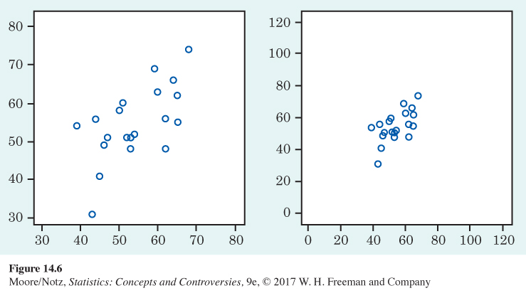
A scatterplot displays the direction, form, and strength of the relationship between two variables. Straight-line relations are particularly important because a straight line is a simple pattern that is quite common. A straight-line relation is strong if the points lie close to a straight line and weak if they are widely scattered about a line. Our eyes are not good judges of how strong a relationship is. The two scatterplots in Figure 14.6 depict the same data, but the right-hand plot is drawn smaller in a large field. The right-hand plot seems to show a stronger straight-line relationship. Our eyes can be fooled by changing the plotting scales or the amount of blank space around the cloud of points in a scatterplot. We need to follow our strategy for data analysis by using a numerical measure to supplement the graph. Correlation is the measure we use.
Correlation
The correlation describes the direction and strength of a straight-line relationship between two quantitative variables. Correlation is usually written as r.
Calculating a correlation takes a bit of work. You can usually think of r as the result of pushing a calculator button or giving a command in software and concentrate on understanding its properties and use. Knowing how we obtain r from data, however, does help us understand how correlation works, so here we go.
EXAMPLE 4 Calculating correlation
We have data on two variables, x and y, for n individuals. For the fossil data in Example 3, x is femur length, y is humerus length, and we have data for n = 5 fossils.
Step 1. Find the mean and standard deviation for both x and y. For the fossil data, a calculator tells us that
| Femur: | ˉx=58.2 cm | sx=13.20 cm |
| Humerus: | ˉy=66.0 cm | sy=15.89 cm |
We use sx and sy to remind ourselves that there are two standard deviations, one for the values of x and the other for the values of y.
Step 2. Using the means and standard deviations from Step 1, find the standard scores for each x-value and for each y-value:
|
Value of x |
Standard score (x−ˉx)/sx |
Value of y |
Standard score (y−ˉy)/sy |
| 38 | (38−58.2)/13.20=−1.530 | 41 | (41−66.0)/15.89=−1.573 |
| 56 | (56−58.2)/13.20=−0.167 | 63 | (63−66.0)/15.89=−0.189 |
| 59 | (59−58.2)/13.20= 0.061 | 70 | (70−66.0)/15.89= 0.252 |
| 64 | (64−58.2)/13.20= 0.439 | 72 | (72−66.0)/15.89= 0.378 |
| 74 | (74−58.2)/13.20= 1.197 | 84 | (84−66.0)/15.89= 1.133 |
Step 3. The correlation is the average of the products of these standard scores. As with the standard deviation, we “average” by dividing by n − 1, one fewer than the number of individuals:
r=14[(−1.530)(−1.573)+(−0.167)(−0.189)+(0.061)(0.252) +(0.439)(0.378)+(1.197)(1.133)]=14(2.4067 + 0.0316 + 0.0154 + 0.1659 + 1.3562)=3.97584=0.994
The algebraic shorthand for the set of calculations in Example 4 is
r=1n−1∑(x−ˉxsx)(y−ˉysy)
The symbol ∑, called “sigma,” means “add them all up.”