Chapter 18: Probability Models

Probability models for sampling

432

Choosing a random sample from a population and calculating a statistic such as the sample proportion is certainly a random phenomenon. The distribution of the statistic tells us what values it can take and how often it takes those values. That sounds a lot like a probability model.

EXAMPLE 3 A sampling distribution

Take a simple random sample of 1015 adults. Ask each whether they feel childhood vaccinations are extremely important. The proportion who say Yes

is the sample proportion . Do this 1000 times and collect the 1000 sample proportions from the 1000 samples. The histogram in Figure 18.2 shows the distribution of 1000 sample proportions when the truth about the population is that 54% would say Yes. The results of random sampling are of course random: we can’t predict the outcome of one sample, but the figure shows that the outcomes of many samples have a regular pattern.

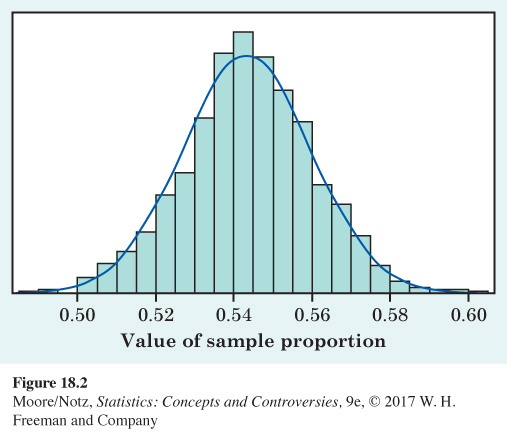
Figure 18.2: Figure 18.2 The sampling distribution of a sample proportion from SRSs of size 1015 drawn from a population in which 54% of the members would give positive answers, Example 3. The histogram shows the distribution from 1000 samples. The Normal curve is the ideal pattern that describes the results of a very large number of samples.

This repetition reminds us that the regular pattern of repeated random samples is one of the big ideas of statistics. The Normal curve in the figure is a good approximation to the histogram. The histogram is the result of these particular 1000 SRSs. Think of the Normal curve as the idealized pattern we would get if we kept on taking SRSs from this population forever. That’s exactly the idea of probability—the pattern we would see in the very long run. The Normal curve assigns probabilities to sample proportions computed from random samples.

433

This Normal curve has mean 0.540 and standard deviation about 0.016. The “95” part of the 68–95–99.7 rule says that 95% of all samples will give a falling within 2 standard deviations of the mean. That’s within 0.032 of 0.540, or between 0.508 and 0.572. We now have more concise language for this fact: the probability is 0.95 that between 50.8% and 57.2% of the people in a sample will say Yes. The word “probability” says we are talking about what would happen in the long run, in very many samples.

We note that of the 1000 SRSs, 95% of the sample proportions were between 0.509 and 0.575, which agrees quite well with the calculations based on the Normal curve. This confirms our assertion that the Normal curve is a good approximation to the histogram in Figure 18.2.

A statistic from a large sample has a great many possible values. Assigning a probability to each individual outcome worked well for four marital classes or 36 outcomes of rolling two dice but is awkward when there are thousands of possible outcomes. Example 3 uses a different approach: assign probabilities to intervals of outcomes by using areas under a Normal density curve. Density curves have area 1 underneath them, which lines up nicely with total probability 1. The total area under the Normal curve in Figure 18.2 is 1, and the area between 0.508 and 0.572 is 0.95, which is the probability that a sample gives a result in that interval. When a Normal curve assigns probabilities, you can calculate probabilities from the 68–95–99.7 rule or from Table B of percentiles of Normal distributions. These probabilities satisfy Rules A through D.

Sampling distribution

The sampling distribution of a statistic tells us what values the statistic takes in repeated samples from the same population and how often it takes those values.

We think of a sampling distribution as assigning probabilities to the values the statistic can take. Because there are usually many possible values, sampling distributions are often described by a density curve such as a Normal curve.

434

Figure 18.3: Figure 18.3 The Normal sampling distribution, Example 4. Because 0.478 is 1 standard deviation below the mean, the area under the curve to the left of 0.478 is 0.16.

EXAMPLE 4 Do you approve of gambling?

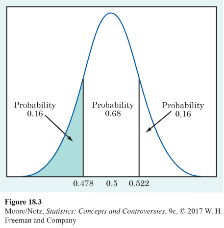
An opinion poll asks an SRS of 501 teens, “Generally speaking, do you approve or disapprove of legal gambling or betting?” Suppose that, in fact, exactly 50% of all teens would say Yes if asked. (This is close to what polls show to be true.) The poll’s statisticians tell us that the sample proportion who say Yes will vary in repeated samples according to a Normal distribution with mean 0.5 and standard deviation about 0.022. This is the sampling distribution of the sample proportion .

The 68–95–99.7 rule says that the probability is 0.16 that the poll gets a sample in which fewer than 47.8% say Yes. Figure 18.3 shows how to get this result from the Normal curve of the sampling distribution.

NOW IT’S YOUR TURN

Question 18.2

18.2 Teen opinion poll. Refer to Example 4. Using the 68–95–99.7 rule, what is the probability that fewer than 45.6% say Yes?

EXAMPLE 5 Using Normal percentiles^*

What is the probability that the opinion poll in Example 4 will get a sample in which 52% or more say Yes? Because 0.52 is not 1, 2, or 3 standard deviations away from the mean, we can’t use the 68–95–99.7 rule. We will use Table B of percentiles of Normal distributions.

435

Figure 18.4: Figure 18.4 The Normal sampling distribution, Example 5. The outcome 0.52 has standard score 0.9, so Table B tells us that the area under the curve to the left of 0.52 is 0.8159.

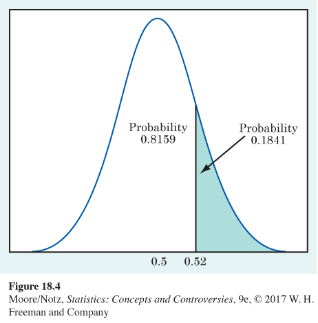
To use Table B, first turn the outcome into a standard score by subtracting the mean of the distribution and dividing by its standard deviation:

Now look in Table B. A standard score of 0.9 is the 81.59 percentile of a Normal distribution. This means that the probability is 0.8159 that the poll gets a smaller result. By Rule C (or just the fact that the total area under the curve is 1), this leaves probability 0.1841 for outcomes with 52% or more answering Yes. Figure 18.4 shows the probabilities as areas under the Normal curve.

*Example 5 is optional.