Expected values
Gambling on chance outcomes goes back to ancient times and has continued throughout history. Both public and private lotteries were common in the early years of the United States. After disappearing for a century or so, government-run gambling reappeared in 1964, when New Hampshire caused a furor by introducing a lottery to raise public revenue without raising taxes. The furor subsided quickly as larger states adopted the idea. Forty-two states and all Canadian provinces now sponsor lotteries. State lotteries made gambling acceptable as entertainment. Some form of legal gambling is allowed in 48 of the 50 states. More than half of all adult Americans have gambled legally. They spend more betting than on spectator sports, video games, theme parks, and movie tickets combined. If you are going to bet, you should understand what makes a bet good or bad. As our introductory Case Study says, we care about how much we win as well as about our probability of winning.
EXAMPLE 1 The Tri-State Daily Numbers
Here is a simple lottery wager: the “Straight” from the Pick 3 game of the Tri-State Daily Numbers offered by New Hampshire, Maine, and Vermont. You pay $0.50 and choose a three-digit number. The state chooses a three-digit winning number at random and pays you $250 if your number is chosen. Because there are 1000 three-digit numbers, you have probability 1-in-1000 of winning. Here is the probability model for your winnings:
| Outcome: | $0 | $250 |
| Probability: | 0.999 | 0.001 |
What are your average winnings? The ordinary average of the two possible outcomes $0 and $250 is $125, but that makes no sense as the average winnings because $250 is much less likely than $0. In the long run, you win $250 once in every 1000 bets and $0 on the remaining 999 of 1000 bets. (Of course, if you play the game regularly, buying one ticket each time you play, after you have bought exactly 1000 Pick 3 tickets, there is no guarantee that you will win exactly once. Probabilities are only long-run proportions.) Your long-run average winnings from a ticket are
$25011000+$09991000=$0.25
or 25 cents. You see that in the long run the state pays out one-half of the money bet and keeps the other half.
Here is a general definition of the kind of “average outcome” we used to evaluate the bets in Example 1.
Expected value
The expected value of a random phenomenon that has numerical outcomes is found by multiplying each outcome by its probability and then adding all the products.
In symbols, if the possible outcomes are a1, a2, . . . , ak and their probabilities are p1, p2, . . . , pk, the expected value is
expected value = a1p1 + a2p2 + · · · + akpk
An expected value is an average of the possible outcomes, but it is not an ordinary average in which all outcomes get the same weight. Instead, each outcome is weighted by its probability so that outcomes that occur more often get higher weights.
EXAMPLE 2 The Tri-State Daily Numbers, continued
The Straight wager in Example 1 pays off if you match the three-digit winning number exactly. You can choose instead to make a $1 StraightBox (six-way) wager. You again choose a three-digit number, but you now have two ways to win. You win $292 if you exactly match the winning number, and you win $42 if your number has the same digits as the winning number, in any order. For example, if your number is 123, you win $292 if the winning number is 123 and $42 if the winning number is any of 132, 213, 231, 312, and 321. In the long run, you win $292 once every 1000 bets and $42 five times for every 1000 bets.
The probability model for the amount you win is
| Outcome: | $0 | $42 | $292 |
| Probability: | 0.994 | 0.005 | 0.001 |
The expected value is
expected value = ($0)(0.994) + ($42)(0.005) + ($292)(0.001) = $0.502
We see that the StraightBox is a slightly better bet than the Straight bet because the state pays out slightly more than half the money bet.
![]() Rigging the lottery We have all seen televised lottery drawings in which numbered balls bubble about and are randomly popped out by air pressure. How might we rig such a drawing? In 1980, the Pennsylvania lottery was rigged by the host and several stagehands. They injected paint into all balls bearing 8 of the 10 digits. This weighed them down and guaranteed that all three balls for the winning number would have the remaining two digits. The perps then bet on all combinations of these digits. When 6-6-6 popped out, they won $1.2 million. Yes, they were caught.
Rigging the lottery We have all seen televised lottery drawings in which numbered balls bubble about and are randomly popped out by air pressure. How might we rig such a drawing? In 1980, the Pennsylvania lottery was rigged by the host and several stagehands. They injected paint into all balls bearing 8 of the 10 digits. This weighed them down and guaranteed that all three balls for the winning number would have the remaining two digits. The perps then bet on all combinations of these digits. When 6-6-6 popped out, they won $1.2 million. Yes, they were caught.
The Tri-State Daily Numbers is unusual among state lottery games in that it pays a fixed amount for each type of bet. Most states pay off on the “pari-mutuel” system. New Jersey’s Pick 3 game is typical: the state pools the money bet and pays out half of it, equally divided among the winning tickets. You still have probability 1-in-1000 of winning a Straight bet, but the amount your number 123 wins depends both on how much was bet on Pick 3 that day and on how many other players chose the number 123. Without fixed amounts, we can’t find the expected value of today’s bet on 123, but one thing is constant: the state keeps half the money bet.
The idea of expected value as an average applies to random outcomes other than games of chance. It is used, for example, to describe the uncertain return from buying stocks or building a new factory. Here is a different example.
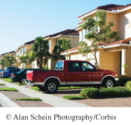
EXAMPLE 3 How many vehicles per household?
What is the average number of motor vehicles in American households? The Census Bureau tells us that the distribution of vehicles per household (based on the 2010 census) is as follows:
| Number of vehicles: | 0 | 1 | 2 | 3 | 4 | 5 |
| Proportion of households: |
0.09 | 0.34 | 0.37 | 0.14 | 0.05 | 0.01 |
This is a probability model for choosing a household at random and counting its vehicles. (We ignored the very few households with more than five vehicles.) The expected value for this model is the average number of vehicles per household. This average is
expected value = (0)(0.09) + (1)(0.34) + (2)(0.37)
+ (3)(0.14) + (4)(0.05) + (5)(0.01)
= 1.75 vehicles per household
NOW IT’S YOUR TURN
Question 20.1
20.1 Number of children. The Census Bureau gives this distribution for the number of a household’s related children under the age of 18 in American households in 2011:
| Number of children: | 0 | 1 | 2 | 3 | 4 |
| Proportion: | 0.67 | 0.14 | 0.12 | 0.05 | 0.02 |
In this table, 4 actually represents four or more. But for purposes of this exercise, assume that it means only households with exactly four children under the age of 18. This is also the probability distribution for the number of children under 18 in a randomly chosen household. The expected value of this distribution is the average number of children under 18 in a household. What is this expected value?
20.1 The expected value is (0)(0.67) + (1)(.14) + (2)(.12) + (3)(.05) + (4)(.02) = 0.61. The average number of children under 18 in a household is 0.61.