The sampling distribution of a sample mean*
What is the mean number of hours your college’s first-year students study each week? What was their mean grade point average in high school? We often want to estimate the mean of a population. To distinguish the population mean (a parameter) from the sample mean ˉx, we write the population mean as μ, the Greek letter mu. We use the mean ˉx of an SRS to estimate the unknown mean μ of the population.
Like the sample proportion ˆp, the sample mean ˉx from a large SRS has a sampling distribution that is close to Normal. Because the sample mean of an SRS is an unbiased estimator of μ, the sampling distribution of ˉx has μ as its mean. The standard deviation, or standard error, of ˉx depends on the standard deviation of the population, which is usually written as σ, the Greek letter sigma. By mathematics we can discover the following facts.
Sampling distribution of a sample mean
Choose an SRS of size n from a population in which individuals have mean μ and standard deviation σ. Let ˉx be the mean of the sample. Then:
• The sampling distribution of ˉx is approximately Normal when the sample size n is large.
• The mean of the sampling distribution is equal to μ.
• The standard deviation or the standard error of the sampling distribution is σ/√n.
It isn’t surprising that the values that ˉx takes in many samples are centered at the true mean μ of the population. That’s the lack of bias in random sampling once again. The other two facts about the sampling distribution make precise two very important properties of the sample mean ˉx:
• The mean of a number of observations is less variable than individual observations.
• The distribution of a mean of a number of observations is more Normal than the distribution of individual observations.
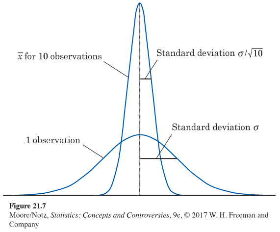
Figure 21.7 illustrates the first of these properties. It compares the distribution of a single observation with the distribution of the mean ˉx of 10 observations. Both have the same center, but the distribution of ˉx is less spread out. In Figure 21.7, the distribution of individual observations is Normal. If that is true, then the sampling distribution of ˉx is exactly Normal for any size sample, not just approximately Normal for large samples. A remarkable statistical fact, called the central limit theorem, says that as we take more and more observations at random from any population, the distribution of the mean of these observations eventually gets close to a Normal distribution. (There are some technical qualifications to this big fact, but in practice, we can ignore them.) The central limit theorem lies behind the use of Normal sampling distributions for sample means.
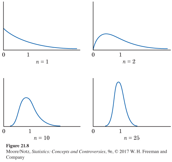
EXAMPLE 6 The central limit theorem in action
Figure 21.8 shows the central limit theorem in action. The top-left density curve describes individual observations from a population. It is strongly right-skewed. Distributions like this describe the time it takes to repair a household appliance, for example. Most repairs are quickly done, but some are lengthy.
The other three density curves in Figure 21.8 show the sampling distributions of the sample means of 2, 10, and 25 observations from this population. As the sample size n increases, the shape becomes more Normal The mean remains fixed and the standard error decreases, following the pattern σ/√n. The distribution for 10 observations is still somewhat skewed to the right but already resembles a Normal curve. The density curve for n = 25 is yet more Normal. The contrast between the shapes of the population distribution and of the distribution of the mean of 10 or 25 observations is striking.
*This section is optional.