Chapter 22: What Is a Test of Significance?

Hypotheses and P-values

Tests of significance refine (and perhaps hide) this basic reasoning. In most studies, we hope to show that some definite effect is present in the population. In Example 1, we suspect that a majority of coffee drinkers prefer fresh-brewed coffee. A statistical test begins by supposing for the sake of argument that the effect we seek is not present. We then look for evidence against this supposition and in favor of the effect we hope to find. The first step in a test of significance is to state a claim that we will try to find evidence against.

Page 525

Null hypothesis H₀

The claim being tested in a statistical test is called the null hypothesis. The test is designed to assess the strength of the evidence against the null hypothesis. Usually, the null hypothesis is a statement of “no effect’’ or “no difference.’’

The term “null hypothesis’’ is abbreviated H₀ and is read as “H-naught,’’ “H-oh,’’ and sometimes even “H-null.’’ It is a statement about the population and so must be stated in terms of a population parameter. In Example 1, the parameter is the proportion p of all coffee drinkers who prefer fresh to instant coffee. The null hypothesis is

H₀: p = 0.5

Gotcha! A tax examiner suspects that Ripoffs, Inc., is issuing phony checks to inflate its expenses and reduce the tax it owes. To learn the truth without examining every check, she boots up her computer. The first digits of real data follow well-known patterns that do not give digits 0 to 9 equal probabilities. If the check amounts don’t follow this pattern, she will investigate. Down the street, a hacker is probing a company’s computer files. He can’t read them because they are encrypted. But he may be able to locate the key to the encryption anyway—if it’s the only long string that really does give equal probability to all possible characters. Both the tax examiner and the hacker need a method for testing whether the pattern they are looking for is present.

The statement we hope or suspect is true instead of H₀ is called the alternative hypothesis and is abbreviated H_a. In Example 1, the alternative hypothesis is that a majority of the population favor fresh coffee. In terms of the population parameter, this is

H_a: p > 0.5

A significance test looks for evidence against the null hypothesis and in favor of the alternative hypothesis. The evidence is strong if the outcome we observe would rarely occur if the null hypothesis is true but is more probable if the alternative hypothesis is true. For example, it would be surprising to find 36 of 50 subjects favoring fresh coffee if, in fact, only half of the population feel this way. How surprising? A significance test answers this question by giving a probability: the probability of getting an outcome at least as far as the actually observed outcome from what we would expect when H₀ is true. What counts as “far from what we would expect’’ depends on H_a as well as H₀. In the taste test, the probability we want is the probability that 36 or more of 50 subjects favor fresh coffee. If the null hypothesis p = 0.5 is true, this probability is very small (0.001). That’s good evidence that the null hypothesis is not true.

Page 526

P-value

The probability, computed assuming that H₀ is true, that the sample outcome would be as extreme or more extreme than the actually observed outcome is called the P-value of the test. The smaller the P-value is, the stronger is the evidence against H₀ provided by the data.

In practice, most statistical tests are carried out by computer software that calculates the P-value for us. It is usual to report the P-value in describing the results of studies in many fields. You should, therefore, understand what P-values say even if you don’t do statistical tests yourself, just as you should understand what “95% confidence’’ means even if you don’t calculate your own confidence intervals.

EXAMPLE 2 Count Buffon’s coin

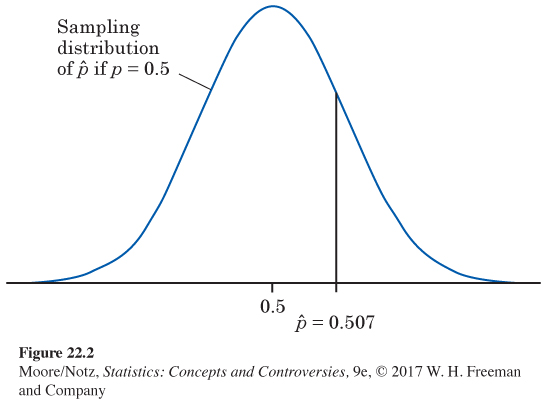
The French naturalist Count Buffon (1707–1788) considered questions ranging from evolution to estimating the number “pi’’ and made it his goal to answer them. One question he explored was whether a “balanced’’ coin would come up heads half of the time when tossed. To investigate, he tossed a coin 4040 times. He got 2048 heads. The sample proportion of heads is

$\hat{p} = \frac{2048}{4040} = 0.507$

That’s a bit more than one-half. Is this evidence that Buffon’s coin was not balanced? This is a job for a significance test.

The hypotheses. The null hypothesis says that the coin is balanced (p = 0.5). We did not suspect a bias in a specific direction before we saw the data, so the alternative hypothesis is just “the coin is not balanced.’’ The two hypotheses are

H₀: p = 0.5

H_a: p ≠ 0.5

The sampling distribution. If the null hypothesis is true, the sample proportion of heads has approximately the Normal distribution with

mean = p = 0.5

$standard deviation = \sqrt{\frac{p (1 - p)}{n}}$

$= \sqrt{\frac{(0.5) (0.5)}{4040}}$

= 0.00786

Page 527

The data. Figure 22.2 shows this sampling distribution with Buffon’s sample outcome $\hat{p} = 0.507$ marked. The picture already suggests that this is not an unlikely outcome that would give strong evidence against the claim that p = 0.5.

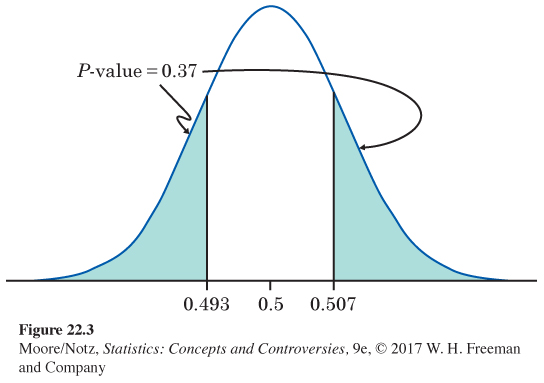
The P-value. How unlikely is an outcome as far from 0.5 as Buffon’s $\hat{p} = 0.507$ ? Because the alternative hypothesis allows p to lie on either side of 0.5, values of $\hat{p}$ far from 0.5 in either direction provide evidence against H₀ and in favor of H_a. The P-value is, therefore, the probability that the observed $\hat{p}$ lies as far from 0.5 in either direction as the observed $\hat{p} = 0.507$ . Figure 22.3 shows this probability as area under the Normal curve. It is P = 0.37.

The conclusion. A truly balanced coin would give a result this far or farther from 0.5 in 37% of all repetitions of Buffon’s trial. His result gives no reason to think that his coin was not balanced.

The alternative H_a: p > 0.5 in Example 1 is a one-sided alternative because the effect we seek evidence for says that the population proportion is greater than one-half. The alternative H_a: p ≠ 0.5 in Example 2 is a two-sided alternative because we ask only whether or not the coin is balanced. Whether the alternative is one-sided or two-sided determines whether sample results that are extreme in one direction or in both directions count as evidence against H₀ in favor of H_a.

Figure 22.2: Figure 22.2 The sampling distribution of the proportion of heads in 4040 tosses of a balanced coin, Example 2. Count Buffon’s result, proportion 0.507 heads, is marked.

Page 528

Figure 22.3: Figure 22.3 The P-value for testing whether Count Buffon’s coin was balanced, Example 2. This is the probability, calculated assuming a balanced coin, of a sample proportion as far or farther from 0.5 as Buffon’s result of 0.507.

NOW IT’S YOUR TURN

Question 22.1

22.1 Coin tossing. We do not have the patience of Count Buffon, so we tossed a coin only 50 times. We got 21 heads. The proportion of heads is

$\hat{p} = \frac{21}{50} = 0.42$

This is less than one-half. Is this evidence that our coin is not balanced? Formulate the hypotheses for an appropriate significance test and determine the sampling distribution of the sample proportion of heads if the null hypothesis is true. As you are working through this problem, think about what you learned in Chapters 17 and 20 about the “law of large numbers.” Does it make sense that your sample proportion would be different with a smaller sample size?

22.1 The hypotheses. The null hypothesis says that the coin is balanced (p = 0.5). We do not suspect a bias in a specific direction before we see the data, so the alternative hypothesis is just “the coin is not balanced.” The two hypotheses are

H₀ : p = 0.5

H_a : p ≠ 0.5

The sampling distribution. If the null hypothesis is true, the sample proportion of heads has approximately the Normal distribution with

mean = p = 0.5

$standard deviation = \sqrt{\frac{p (1 - p)}{n}}$

$= \sqrt{\frac{(0.5) (0.5)}{50}}$

= 0.0707