Chapter 23: Use and Abuse of Statistical Inference

The woes of significance tests

The purpose of a significance test is usually to give evidence for the presence of some effect in the population. The effect might be a probability of heads different from one-half for a coin or a longer mean survival time for patients given a new cancer treatment. If the effect is large, it will show up in most samples—the proportion of heads among our tosses will be far from one-half, or the patients who get the new treatment will live much longer than those in the control group. Small effects, such as a probability of heads only slightly different from one-half, will often be hidden behind the chance variation in a sample. This is as it should be: big effects are easier to detect. That is, the P-value will usually be small when the population truth is far from the null hypothesis.

The “woes” of testing start with the fact that a test measures only the strength of evidence against the null hypothesis. It says nothing about how big or how important the effect we seek in the population really is. For example, our hypothesis might be “This coin is balanced.” We express this hypothesis in terms of the probability p of getting a head as H₀: p = 0.5. No real coin is exactly balanced, so we know that this hypothesis is not exactly true. If this coin has probability p = 0.502 of a head, we might say that, for practical purposes, it is balanced. A statistical test doesn’t think about “practical purposes.” It just asks if there is evidence that p is not exactly equal to 0.5. The focus of tests on the strength of the evidence against an exact null hypothesis is the source of much confusion in using tests.

551

Pay particular attention to the size of the sample when you read the result of a significance test. Here’s why:

• Larger samples make tests of significance more sensitive. If we toss a coin hundreds of thousands of times, a test of H₀: p = 0.5 will often give a very low P-value when the truth for this coin is p = 0.502. The test is right—it found good evidence that p really is not exactly equal to 0.5—but it has picked up a difference so small that it is of no practical interest. A finding can be statistically significant without being practically important.
• On the other hand, tests of significance based on small samples are often not sensitive. If you toss a coin only 10 times, a test of H₀: p = 0.5 will often give a large P-value even if the truth for this coin is p = 0.7. Again the test is right—10 tosses are not enough to give good evidence against the null hypothesis. Lack of significance does not mean that there is no effect, only that we do not have good evidence for an effect. Small samples often miss important effects that are really present in the population. As cosmologist Martin Rees said, “Absence of evidence is not evidence of absence.”

EXAMPLE 2 Antidepressants versus a placebo

Through a Freedom of Information Act request, two psychologists obtained 47 studies used by the Food and Drug Administration for approval of the six antidepressants prescribed most widely between 1987 and 1999. Overall, the psychologists found that there was a statistically significant difference in the effects of antidepressants compared with a placebo, with antidepressants being more effective. However, the psychologists went on to report that antidepressant pills worked 18% better than placebos, a statistically significant difference, “but not meaningful for people in clinical settings.’’

Whatever the truth about the population, whether p = 0.7 or p = 0.502, more observations allow us to estimate p more closely. If p is not 0.5, more observations will give more evidence of this, that is, a smaller P-value. Because statistical significance depends strongly on the sample size as well as on the truth about the population, statistical significance tells us nothing about how large or how practically important an effect is. Large effects (like p = 0.7 when the null hypothesis is p = 0.5) often give data that are insignificant if we take only a small sample. Small effects (like p = 0.502) often give data that are highly significant if we take a large enough sample. Let’s return to a favorite example to see how significance changes with sample size.

552

EXAMPLE 3 Count Buffon’s coin again

Count Buffon tossed a coin 4040 times and got 2048 heads. His sample proportion of heads was

Is the count’s coin balanced? Suppose we seek statistical significance at level 0.05. The hypotheses are

H₀: p = 0.5

H_a: p ≠ 0.5

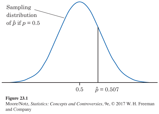
The test of significance works by locating the sample outcome = 0.507 on the sampling distribution that describes how would vary if the null hypothesis were true. Figure 23.1 repeats Figure 22.2. It shows that the observed = 0.507 is not surprisingly far from 0.5 and, therefore, is not good evidence against the hypothesis that the true p is 0.5. The P-value, which is 0.37, just makes this precise.

Figure 23.1: Figure 23.1 The sampling distribution of the proportion of heads in 4040 tosses of a coin if in fact the coin is balanced, Example 3. Sample proportion 0.507 is not an unusual outcome.

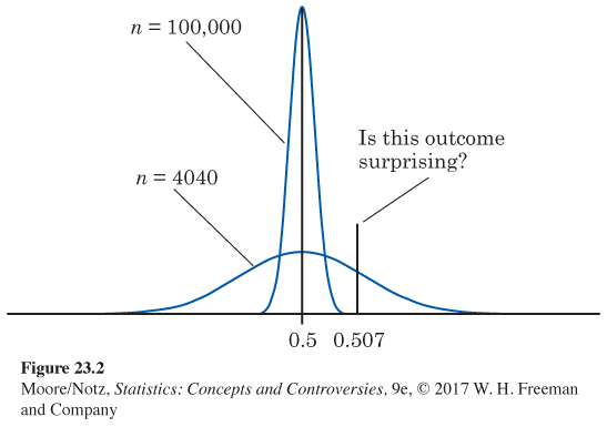
Suppose that Count Buffon got the same result, = 0.507, from tossing a coin 100,000 times. The sampling distribution of when the null hypothesis is true always has mean 0.5, but its standard deviation gets smaller as the sample size n gets larger. Figure 23.2 displays the two sampling distributions, for n = 4040 and n = 100,000. The lower curve in this figure is the same Normal curve as in Figure 23.1, drawn on a scale that allows us to show the very tall and narrow curve for n = 100,000. Locating the sample outcome = 0.507 on the two curves, you see that the same outcome is more or less surprising depending on the size of the sample.

553

Figure 23.2: Figure 23.2 The two sampling distributions of the proportion of heads in 4040 and 100,000 tosses of a balanced coin, Example 3. Sample proportion 0.507 is not unusual in 4040 tosses but is very unusual in 100,000 tosses.

The P-values are P = 0.37 for n = 4040 and P = 0.000009 for n = 100,000. Imagine tossing a balanced coin 4040 times repeatedly. You will get a proportion of heads at least as far from one-half as Buffon’s 0.507 in about 37% of your repetitions. If you toss a balanced coin 100,000 times repeatedly, however, you will almost never (nine times in one million repeats) get an outcome as or more unbalanced than this.

The outcome = 0.507 is not evidence against the hypothesis that the coin is balanced if it comes up in 4040 tosses. It is completely convincing evidence if it comes up in 100,000 tosses.

Beware the naked P-value

The P-value of a significance test depends strongly on the size of the sample, as well as on the truth about the population.

It is bad practice to report a naked P-value (a P-value by itself) without also giving the sample size and a statistic or statistics that describe the sample outcome.

554

NOW IT’S YOUR TURN

Question 23.1

23.1 Weight loss. A company that sells a weight-loss program conducted a randomized experiment to determine whether people lost weight after eight weeks on the program. The company researchers report that, on average, the subjects in the study lost weight and that the weight loss was statistically significant with a P-value of 0.013. Do you find the results convincing? If so, why? If not, what additional information would you like to have?