Tests of significance were presented in Chapter 22 as methods for assessing the strength of evidence against the null hypothesis. The assessment is made by the P-value, which is the probability computed under the assumption that the null hypothesis is true. The alternative hypothesis (the statement we seek evidence for) enters the test only to help us see what outcomes count against the null hypothesis. Such is the theory of tests of significance as advocated by Sir Ronald A. Fisher and as practiced by many users of statistics.

558

But we have also seen signs of another way of thinking in Chapter 22. A level of significance α chosen in advance points to the outcome of the test as a decision. If the P-value is less than α, we reject H₀ in favor of H_a; otherwise we fail to reject H₀. The transition from measuring the strength of evidence to making a decision is not a small step. It can be argued (and is argued by followers of Fisher) that making decisions is too grand a goal, especially in scientific inference. A decision is reached only after the evidence of many experiments is weighed, and indeed the goal of research is not “decision” but a gradually evolving understanding. Better that statistical inference should content itself with confidence intervals and tests of significance. Many users of statistics are content with such methods. It is rare (outside textbooks) to set up a level α in advance as a rule for decision making in a scientific problem. More commonly, users think of significance at level 0.05 as a description of good evidence. This is made clearer by talking about P-values, and this newer language is spreading.

Yet there are circumstances in which a decision or action is called for as the end result of inference. Acceptance sampling is one such circumstance. The supplier of a product (for example, potatoes to be used to make potato chips) and the consumer of the product agree that each truckload of the product shall meet certain quality standards. When a truckload arrives, the consumer chooses a sample of the product to be inspected. On the basis of the sample outcome, the consumer will either accept or reject the truckload. Fisher agreed that this is a genuine decision problem. But he insisted that acceptance sampling is completely different from scientific inference. Other eminent statisticians have argued that if “decision’’ is given a broad meaning, almost all problems of statistical inference can be posed as problems of making decisions in the presence of uncertainty. We are not going to venture further into the arguments over how we ought to think about inference. We do want to show how a different concept—inference as decision—changes the ways of reasoning used in tests of significance.

Tests of significance fasten attention on H₀, the null hypothesis. If a decision is called for, however, there is no reason to single out H₀. There are simply two alternatives, and we must accept one and reject the other. It is convenient to call the two alternatives H₀ and H_a, but H₀ no longer has the special status (the statement we try to find evidence against) that it had in tests of significance. In the acceptance sampling problem, we must decide between

H₀: the truckload of product meets standards

H_a: the truckload does not meet standards

559

on the basis of a sample of the product. There is no reason to put the burden of proof on the consumer by accepting H₀ unless we have strong evidence against it. It is equally sensible to put the burden of proof on the producer by accepting H_a unless we have strong evidence that the truckload meets standards. Producer and consumer must agree on where to place the burden of proof, but neither H₀ nor H_a has any special status.

In a decision problem, we must give a decision rule—a recipe based on the sample that tells us what decision to make. Decision rules are expressed in terms of sample statistics, usually the same statistics we would use in a test of significance. In fact, we have already seen that a test of significance becomes a decision rule if we reject H₀ (accept H_a) when the sample statistics is statistically significant at level α and otherwise accept H₀ (reject H_a).

Suppose, then, that we use statistical significance at level α as our criterion for decision. And suppose that the null hypothesis H₀ is really true. Then, sample outcomes significant at level α will occur with probability α. (That’s the definition of “significant at level α”; outcomes weighing strongly against H₀ occur with probability α when H₀ is really true.) But now we make a wrong decision in all such outcomes, by rejecting H₀ when it is really true. That is, significance level α now can be understood as the probability of a certain type of wrong decision.

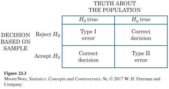
Now H_a requires equal attention. Just as rejecting H₀ (accepting H_a) when H₀ is really true is an error, so is accepting H₀ (rejecting H_a) when H_a is really true. We can make two kinds of errors.

The possibilities are summed up in Figure 23.3. If H₀ is true, our decision is either correct (if we accept H_a) or is a Type I error. Only one error is possible at one time. Figure 23.4 applies these ideas to the acceptance sampling example.

560

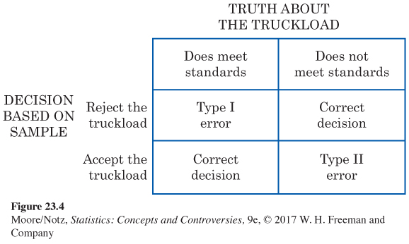
So the significance level α is the probability of a Type I error. In acceptance sampling, this is the probability that a good truckload will be rejected. The probability of a Type II error is the probability that a bad truckload will be accepted. A Type I error hurts the producer, while a Type II error hurts the consumer. Any decision rule is assessed in terms of the probabilities of the two types of error. This is in keeping with the idea that statistical inference is based on probability. We cannot (short of inspecting the whole truckload) guarantee that good lots will never be rejected and bad lots never accepted. But by random sampling and the laws of probability, we can say what the probabilities of both kinds of errors are. Because we can find out the monetary cost of accepting bad truckloads and rejecting good ones, we can determine how much loss the producer and consumer each will suffer in the long run from wrong decisions.

Advocates of decision theory argue that the kind of “economic” thinking natural in acceptance sampling applies to all inference problems. Even a scientific researcher decides whether to announce results, or to do another experiment, or to give up research as unproductive. Wrong decisions carry costs, though these costs are not always measured in dollars. A scientist suffers by announcing a false effect, and also by failing to detect a true effect. Decision theorists maintain that the scientist should try to give numerical weights (called utilities) to the consequences of the two types of wrong decision. Then the scientist can choose a decision rule with the error probabilities that reflect how serious the two kinds of error are. This argument has won favor where utilities are easily expressed in money. Decision theory is widely used by business in making capital investment decisions, for example. But scientific researchers have been reluctant to take this approach to statistical inference.

561

To sum up, in a test of significance, we focus on a single hypothesis (H₀) and single probability (the P-value). The goal is to measure the strength of the sample evidence against H₀. If the same inference problem is thought of as a decision problem, we focus on two hypotheses and give a rule for deciding between them based on sample evidence. Therefore, we must focus on two probabilities: the probabilities of the two types of error.

Such a clear distinction between the two types of thinking is helpful for understanding. In practice, the two approaches often merge, to the dismay of partisans of one or the other. We continued to call one of the hypotheses in a decision problem H₀. In the common practice of testing hypotheses, we mix significance tests and decision rules as follows.

Testing hypotheses may seen to be a hybrid approach. It was, historically, the effective beginning of decision-oriented ideas in statistics. Hypothesis testing was developed by Jerzey Neyman^* and Egon S. Pearson in the years 1928–1938. The decision theory approach came later (1940s) and grew out of the Neyman-Pearson ideas. Because decision theory in its pure form leaves you with two error probabilities and no simple rule on how to balance them, it has been used less often than tests of significance. Decision theory ideas have been applied in testing problems mainly by way of the Neyman-Pearson theory. That theory asks you to first choose α, and the influence of Fisher often has led users of hypothesis testing comfortably back to α = 0.05 or α = 0.01 (and also back to the warnings in this chapter about this state of affairs). Fisher, who was exceedingly argumentative, violently attacked the Neyman-Pearson decision-oriented ideas, and the argument still continues.

The reasoning of statistical inference is subtle, and the principles at issue are complex. We have (believe it or not) oversimplified the ideas of all the viewpoints mentioned and omitted several other viewpoints altogether. If you are feeling that you do not fully grasp all of the ideas of this chapter and of Chapter 22, you are in excellent company. Nonetheless, any user of statistics should make a serious effort to grasp the conflicting views on the nature of statistical inference. More than most other kinds of intellectual exercise, statistical inference can be done automatically, by recipe or by computer. These valuable shortcuts are of no worth without understanding. What Euclid said of his own science to King Ptolemy of Egypt long ago remains true of all knowledge: “There is no royal road to geometry.’’

562