Chapter 24: Two-Way Tables and the Chi-Square Test*

The chi-square test

To see if the data give evidence against the null hypothesis of “no relationship,’’ compare the counts in the two-way table with the counts we would expect if there really were no relationship. If the observed counts are far from the expected counts, that’s the evidence we were seeking. The significance test uses a statistic that measures how far apart the observed and expected counts are.

More chi-square tests There are also chi-square tests for hypotheses more specific than “no relationship.’’ Place people in classes by social status, wait 10 years, then classify the same people again. The row and column variables are the classes at the two times. We might test the hypothesis that there has been no change in the overall distribution of social status. Or we might ask if moves up in status are balanced by matching moves down. These hypotheses can be tested by variations of the chi-square test.

Chi-square statistic

The chi-square statistic, denoted $χ^{2}$ , is a measure of how far the observed counts in a two-way table are from the expected counts. The formula for the statistic is

$χ^{2} = {\sum \frac{(observed count − expected count)}{expected count}}^{2}$

The symbol Σ means “sum over all cells in the table.”

The chi-square statistic is a sum of terms, one for each cell in the table. In the cocaine example, 14 of the desipramine group succeeded. The expected count for this cell is 8. So the term in the chi-square statistic from this cell is

$\begin{array}{l} \frac{{(observed count - expected count)}^{2}}{expected count} & = & \frac{{(14 - 8)}^{2}}{8} \\ = & \frac{36}{8} = 4.5 \end{array}$

EXAMPLE 4 The cocaine study

Here are the observed and expected counts for the cocaine study side by side:

	Observed		Expected
	Success	Failure	Success	Failure
Desipramine	14	10	8	16
Lithium	6	18	8	16
Placebo	4	20	8	16

Page 578

We can now find the chi-square statistic, adding six terms for the six cells in the two-way table:

$\begin{array}{l} χ^{2} & = & \frac{{(14 - 8)}^{2}}{8} + \frac{{(10 - 16)}^{2}}{16} + \frac{{(6 - 8)}^{2}}{8} \\ + \frac{{(18 - 16)}^{2}}{16} + \frac{{(4 - 8)}^{2}}{8} + \frac{{(20 - 16)}^{2}}{16} \\ = & 4.50 + 2.25 + 0.50 + 0.25 + 2.00 + 1.00 = 10.50 \end{array}$

NOW IT’S YOUR TURN

Question 24.2

24.2 Video-gaming and grades. The popularity of computer, video, online, and virtual reality games has raised concerns about their ability to negatively impact youth. Based on a recent survey, 1808 students aged 14 to 18 in Connecticut high schools were classified by their average grades and by whether they had or had not played such games. The following table summarizes the findings. The observed and expected counts are given side by side.

	Observed			Expected
	A’s and B’s	C’s	D’s and F’s	A’s and B’s	C’s	D’s and F’s
Played games	736	450	193	717.7	453.1	208.2
Never played games	205	144	80	223.3	140.9	64.8

Find the chi-square statistic.

24.2 To find the chi-square statistic, we add six terms for the six cells in the two-way table:

$\begin{array}{l} X^{2} & = & \frac{{(736 - 717.7)}^{2}}{717.7} + \frac{{(450 - 453.1)}^{2}}{453.1} \\ + \frac{{(193 - 208.2)}^{2}}{208.2} + \frac{{(205 - 223.3)}^{2}}{223.3} \\ + \frac{{(144 - 140.9)}^{2}}{140.9} + \frac{{(80 - 64.8)}^{2}}{64.8} \\ = & 0.47 + 0.02 + 1.11 + 1.50 + 0.07 + 3.57 = 6.74 \end{array}$

Because $χ^{2}$ measures how far the observed counts are from what would be expected if $H_{0}$ were true, large values are evidence against $H_{0}$ . Is $χ^{2} = 10.5$ a large value? You know the drill: compare the observed value 10.5 against the sampling distribution that shows how $χ^{2}$ would vary if the null hypothesis were true. This sampling distribution is not a Normal distribution. It is a right-skewed distribution that allows only non-negative values because $χ^{2}$ can never be negative. Moreover, the sampling distribution is different for two-way tables of different sizes. Here are the facts.

The chi-square distributions

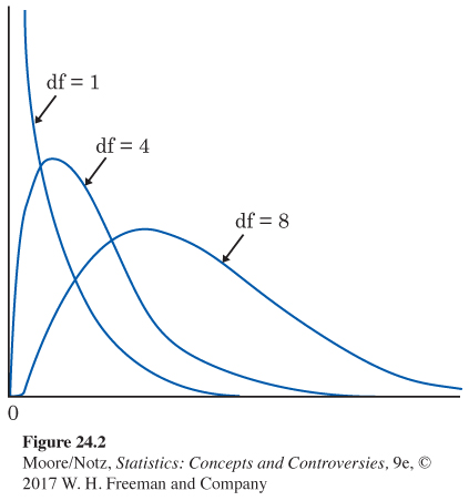
The sampling distribution of the chi-square statistic $χ^{2}$ when the null hypothesis of no association is true is called a chi-square distribution.

Page 579

The chi-square distributions are a family of distributions that take only non-negative values and are skewed to the right. A specific chi-square distribution is specified by giving its degrees of freedom.

The chi-square test for a two-way table with $r$ rows and $c$ columns uses critical values from the chi-square distribution with $(r - 1) (c - 1)$ degrees of freedom.

Figure 24.2 shows the density curves for three members of the chi-square family of distributions. As the degrees of freedom (df) increase, the density curves become less skewed and larger values become more probable. We can’t find $P$ -values as areas under a chi-square curve by hand, though software can do it for us. Table 24.1 is a shortcut. It shows how large the chi-square statistic $χ^{2}$ must be in order to be significant at various levels. This isn’t as good as an actual $P$ -value, but it is often good enough. Each number of degrees of freedom has a separate row in the table. We see, for example, that a chi-square statistic with 3 degrees of freedom is significant at the 5% level if it is greater than 7.81 and is significant at the 1% level if it is greater than 11.34.

EXAMPLE 5 The cocaine study, conclusion

We have seen that desipramine produced markedly more successes and fewer failures than lithium or a placebo. Comparing observed and expected counts gave the chi-square statistic $χ^{2}$ = 10.5. The last step is to assess significance.

Figure 24.2: Figure 24.2 The density curves for three members of the chi-square family of distributions. The sampling distributions of chi-square statistics belong to this family.

Page 580

Table : TABLE 24.1 To be significant at level α, a chi-square statistic must be larger than the table entry for α

	Significance Level α
df	0.25	0.20	0.15	0.10	0.05	0.01	0.001
1	1.32	1.64	2.07	2.71	3.84	6.63	10.83
2	2.77	3.22	3.79	4.61	5.99	9.21	13.82
3	4.11	4.64	5.32	6.25	7.81	11.34	16.27
4	5.39	5.99	6.74	7.78	9.49	13.28	18.47
5	6.63	7.29	8.12	9.24	11.07	15.09	20.51
6	7.84	8.56	9.45	10.64	12.59	16.81	22.46
7	9.04	9.80	10.75	12.02	14.07	18.48	24.32
8	10.22	11.03	12.03	13.36	15.51	20.09	26.12
9	11.39	12.24	13.29	14.68	16.92	21.67	27.88

The two-way table of three treatments by two outcomes for the cocaine study has three rows and two columns. That is, r = 3 and c = 2. The chi-square statistic, therefore, has degrees of freedom

(r − 1)(c −1) = (3 − 1)(2 −1) = (2)(1) = 2

Look in the df = 2 row of Table 24.1. We see that x²= 10.5 is larger than the critical value 9.21 required for significance at the ɑ = 0.01 level but smaller than the critical value 13.82 for ɑ = 0.001. The cocaine study shows a significant relationship ( $P < 0.01$ ) between treatment and success.

The significance test says only that we have strong evidence of some association between treatment and success. We must look at the two-way table to see the nature of the relationship: desipramine works better than the other treatments.

NOW IT’S YOUR TURN

Question 24.3

24.3 Video-gaming and grades. The popularity of computer, video, online, and virtual reality games has raised concerns about their ability to negatively impact youth. Based on a recent survey, 1808 students aged 14 to 18 in Connecticut high schools were classified by their average grades and by whether they had or had not played such games. The following table summarizes the findings. The observed and expected counts are given side by side.

Page 581

	Observed			Expected
	A’s and B’s	C’s	D’s and F’s	A’s and B’s	C’s	D’s and F’s
Played games	736	450	193	717.7	453.1	208.2
Never played games	205	144	80	223.3	140.9	64.8

From these counts, we find that the chi-square statistic is 6.74. Does the study show that there is a statistically significant relationship between playing games and average grades? Use a significance level of 0.05.

24.3 To assess the statistical significance, we begin by noting that the two-way table has two rows and two columns. That is, r = 2 and c = 2. The chi-square statistic therefore has degrees of freedom

(r − 1)(c −1) = (2 − 1)(2 − 1) = (1)(1) = 1

Look in the df = 1 row of Table 24.1. We see that X² = 6.74 is larger than the critical value 3.84 required for significance at the α = 0.05 level. The study shows a significant relationship (P < 0.05) between playing games and average grades.