Sampling variability
If Gallup took a second random sample of 1015 adults, the new sample would have different people in it. It is almost certain that there would not be exactly 548 respondents who feel that childhood vaccines are extremely important. That is, the value of the statistic ˆp will vary from sample to sample. Could it happen that one random sample finds that 54% of American adults feel childhood vaccines are extremely important and a second random sample finds that only 41% feel the same? Random samples eliminate bias from the act of choosing a sample, but they can still be wrong because of the variability that results when we choose at random. If the variation when we take repeated samples from the same population is too great, we can’t trust the results of any one sample.
We are saved by the second great advantage of random samples. The first advantage is that choosing at random eliminates favoritism. That is, random sampling attacks bias. The second advantage is that if we took lots of random samples of the same size from the same population, the variation from sample to sample would follow a predictable pattern. This predictable pattern shows that results of bigger samples are less variable than results of smaller samples.
EXAMPLE 2 Lots and lots of samples
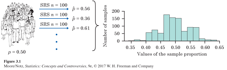
Here’s another big idea of statistics: to see how trustworthy one sample is likely to be, ask what would happen if we took many samples from the same population. Let’s try it and see. Suppose that, in fact (unknown to Gallup), exactly 50% of all American adults feel childhood vaccines are extremely important. That is, the truth about the population is that p = 0.5. What if Gallup used the sample proportion ˆp from an SRS of size 100 to estimate the unknown value of the population proportion p?
Figure 3.1 illustrates the process of choosing many samples and finding ˆp for each one. In the first sample, 56 of the 100 people felt childhood vaccines are extremely important, so ˆp=56/100=0.56. Only 36 in the next sample felt childhood vaccines are extremely important, so for that sample ˆp = 0.36. Choose 1000 samples and make a plot of the 1000 values of ˆp like the graph (called a histogram) at the right of Figure 3.1. The different values of the sample proportion ˆp run along the horizontal axis. The height of each bar shows how many of our 1000 samples gave the group of values on the horizontal axis covered by the bar. For example, in Figure 3.1 the bar covering the values between 0.40 and 0.42 has a height of slightly over 50. Thus, more than 50 of our 1000 samples had values between 0.40 and 0.42.
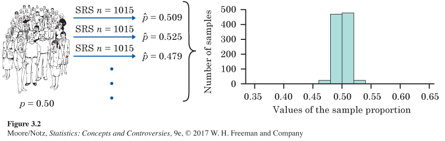
Of course, Gallup interviewed 1015 people, not just 100. Figure 3.2 shows the results of 1000 SRSs, each of size 1015, drawn from a population in which the true sample proportion is p = 0.5. Figures 3.1 and 3.2 are drawn on the same scale. Comparing them shows what happens when we increase the size of our samples from 100 to 1015.
Look carefully at Figures 3.1 and 3.2. We flow from the population, to many samples from the population, to the many values of ˆp from these many samples. Gather these values together and study the histograms that display them.
• In both cases, the values of the sample proportion ˆp vary from sample to sample, but the values are centered at 0.5. Recall that p = 0.5 is the true population parameter. Some samples have a ˆp less than 0.5 and some greater, but there is no tendency to be always low or always high. That is, ˆp has no bias as an estimator of p. This is true for both large and small samples.
• The values of ˆp from samples of size 100 are much more variable than the values from samples of size 1015. In fact, 95% of our 1000 samples of size 1015 have a ˆp lying between 0.4692 and 0.5308. That’s within 0.0308 on either side of the population truth 0.5. Our samples of size 100, on the other hand, spread the middle 95% of their values between 0.40 and 0.60. That goes out 0.10 from the truth, about three times as far as the larger samples. So larger random samples have less variability than smaller samples.
The result is that we can rely on a sample of size 1015 to almost always give an estimate ˆp that is close to the truth about the population. Figure 3.2 illustrates this fact for just one value of the population proportion, but it is true for any population proportion. Samples of size 100, on the other hand, might give an estimate of 40% or 60% when the truth is 50%.
Thinking about Figures 3.1 and 3.2 helps us restate the idea of bias when we use a statistic like ˆp to estimate a parameter like p. It also reminds us that variability matters as much as bias.
Two types of error in estimation
Bias is consistent, repeated deviation of the sample statistic from the population parameter in the same direction when we take many samples. In other words, bias is a systematic overestimate or underestimate of the population parameter.
Variability describes how spread out the values of the sample statistic are when we take many samples. Large variability means that the result of sampling is not repeatable.
A good sampling method has both small bias and small variability.
We can think of the true value of the population parameter as the bull’s-eye on a target and of the sample statistic as an arrow fired at the bull’s-eye. Bias and variability describe what happens when an archer fires many arrows at the target. Bias means that the aim is off, and the arrows land consistently off the bull’s-eye in the same direction. The sample values do not center about the population value. Large variability means that repeated shots are widely scattered on the target. Repeated samples do not give similar results but differ widely among themselves. Figure 3.3 shows this target illustration of the two types of error.
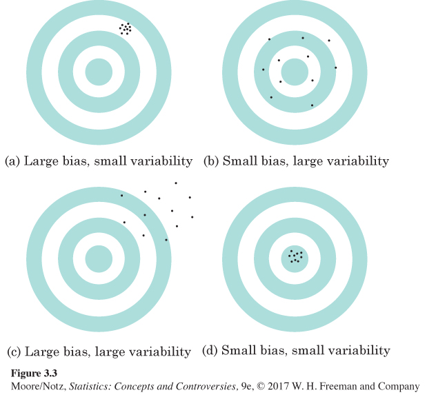
Notice that small variability (repeated shots are close together) can accompany large bias (the arrows are consistently away from the bull’s-eye in one direction). And small bias (the arrows center on the bull’s-eye) can accompany large variability (repeated shots are widely scattered). A good sampling scheme, like a good archer, must have both small bias and small variability. Here’s how we do this:
Managing bias and variability
To reduce bias, use random sampling. When we start with a list of the entire population, simple random sampling produces unbiased estimates: the values of a statistic computed from an SRS neither consistently overestimate nor consistently underestimate the value of the population parameter.
To reduce the variability of an SRS, use a larger sample. You can make the variability as small as you want by taking a large enough sample.
In practice, Gallup takes only one sample. We don’t know how close to the truth an estimate from this one sample is because we don’t know what the truth about the population is. But large random samples almost always give an estimate that is close to the truth. Looking at the pattern of many samples shows how much we can trust the result of one sample.