16.3 The Description of Data

In addition to using graphs and charts, psychologists can describe their data sets using numbers that express important characteristics: measures of central tendency, measures of variation, and measures of position. These numbers are an important component of descriptive statistics, as they provide a current snapshot of a data set.

Measures of Central Tendency

If you want to understand human behaviors and mental processes, it helps to know what is typical, or standard, for the population. What is the average level of intelligence? At what age do most people experience first love? To answer these types of questions, psychologists can describe their data sets by calculating measures of central tendency, which are numbers representing the “middle” of data sets. There are several ways of doing this. The mean is the arithmetic average of a data set. Most students learn how to calculate a mean, or “average,” early in their schooling, using the following formula:

or

To calculate the sample mean for minutes of REM sleep, you would just plug the numbers into the formula:

Another measure of central tendency is the median—the number that represents the position in the middle of the data set. In other words, 50% of the data values are greater than the median, and 50% are smaller. To calculate the median for a small set of numbers, start by ordering the values, and then determine which number lies exactly in the center. This is relatively simple when the data set is odd-numbered; all you have to do is find the value that has the same number of values above and below it. For a data set that has an even number of values, however, there is one additional step: You must take the average of the two middle numbers (add them together and divide by 2). With an odd number of values in a data set, the median will always be a member of the set. With an even number of values, the median may or may not be a member of the data set.

Here is how you would determine the median (Mdn) for the minutes of REM sleep:

1. Order the numbers in the data set from smallest to largest. We can use the stem-and-leaf plot for this purpose.
2. Find the value in the data set that has 50% of the other values below it and 50% above it. Because we have an even number for our sample size (n = 44), we will have to find the middle two data values and calculate their average. We divide our sample size of 44 by 2, which is 22, indicating that the median is midway between the 22nd and 23rd values in our set. We count (starting at 18 in the stem-and-leaf plot) to the 22nd and 23rd numbers in our ordered list (76 and 77; there are 21 values below 76 and 21 values above 77).
3. 

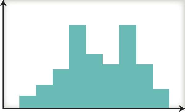
The third common measure of central tendency is the mode, which is the most frequently occurring value in a data set. If there is only one such value, we call it a unimodal distribution. With a symmetric distribution, the mean, median, and mode are the same (see Figure A.4a on page A-6). Sometimes there are two modes, indicating a bimodal distribution, and the shape of the distribution exhibits two vertical bars of equal height (Figure A.8). In our example of REM minutes, we cannot see a clear mode, as there are several values that have a frequency of 2 (35, 47, 49, 68, and 81 minutes). By the way, the mode often provides a better representation of the central tendency with bimodal distributions, because neither the mean nor median will indicate that there are in essence two “centers” for the data set.

Bimodal distribution

Under other circumstances, the median is better than the mean for representing the middle of the data set. This is especially true when the data set includes one or more outliers, or values that are very different from the rest of the set. We can see why this is true by replacing just one value in our data set on REM sleep. See what happens to the mean and median when you swap 150 for 400. First calculate the mean:

1. 
2. And now calculate the median. The numbers in the data set are ordered from smallest to largest. The middle two values have not changed (76 and 77).
   Mdn = 76.5 minutes (identical to the original median of 76.5)

No matter how large (or small) a single value is, it does not change the median, but it can have a great influence on the mean. When this occurs, psychologists often present both of these statistics, and discuss the possibility that an outlier is pulling the mean toward it. Look again at the skewed distributions in Figure A.5 on page A-7 and see how the mean is “pulled” toward the side of the distribution that has a possible outlier in its tail. Some types of data are predictably skewed in one direction or the other. For example, income data collected from populations are often positively skewed. The small proportion of very wealthy people pulls the tail of the distribution to the right. A common example for negatively skewed data is age at retirement, because the great majority of people do not retire until they are in their sixties. In either case, when data are skewed, it is often a good idea to use the median as a measure of central tendency, particularly if a problem exists with outliers.

Measures of Variation

In addition to providing information on the central tendency, psychologists can also use measures of variation to describe how much variation or dispersion there is in a data set. If you look at the two data sets in Figure A.9 (number of miles commuting to school), you can see that they have the same central tendency (identical means: the mean commute for both samples is 30 miles; = 30.0), yet their dispersion is very different: One data set looks very closely packed, and the other spread out.

Same mean, different variability for Sample A and Sample B

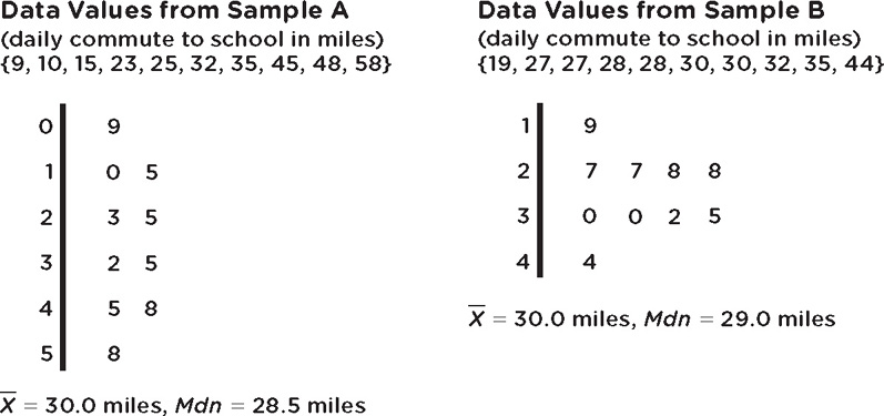
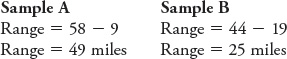
Thus, in addition to knowing the central tendency of a data set, it is also important to describe its variability, or how spread out or dispersed it is. There are several measures we can use to characterize the variability or variation of a data set. The range represents the length of a data set and is calculated by taking the highest value minus the lowest value. The range is a rough depiction of variability, but a useful value for trying to compare two samples with data on the same variable. For the data sets presented in Figure A.9, we can compare the ranges of the two samples and see that Sample A has a range of 49 miles and Sample B has a smaller range of 25 miles.

A more precise measure of dispersion is the standard deviation (referred to by the symbol s when describing samples), which essentially represents the average amount the data points are away from their mean. Think about it like this: If the values in a data set are very close to each other, they will also be very close to their mean, and the dispersion will be small. Their average distance from the mean is small. If the values are widely spread, they will not all be clustered around the mean, and their dispersion will be great. Their average distance from the mean is large. One way we can calculate the standard deviation of a sample is by using the following formula:

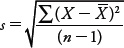
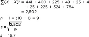
This formula does the following: (1) Subtract the mean from a value in the data set, then square the result. Do this for every value in the data set and take the sum of the results. (2) Divide this sum by the sample size minus 1. (3) Take the square root of the result. In TABLE a.4, we have gone through each of these steps for Sample A.

Table : TABLE A.4 STANDARD DEVIATION FOR SAMPLE A

X
9	9 − 30 = −21	−212 = 441
10	10 − 30 = −20	−202 = 400
15	15 − 30 = −15	−152 = 225
23	23 − 30 = −7	−72 = 49
25	25 − 30 = −5	−52 = 25
32	32 − 30 = 2	22 = 4
35	35 − 30 = 5	52 = 25
45	45 − 30 = 15	152 = 225
48	48 − 30 = 18	182 = 324
58	58 − 30 = 28	282 = 784

The standard deviation for Sample A is 16.7 miles and the standard deviation for Sample B is 6.4 miles (the calculation is not shown here). These standard deviations are consistent with what we expect from looking at the stem-and-leaf plots in Figure A.9. Sample A is more variable, or spread out, than Sample B.

The standard deviation is useful for making predictions about the probability of a particular value occurring Figure A.4b on page A-6. The empirical rule tells us that we can expect approximately 68% of all values to fall within 1 standard deviation below or above their mean. We can expect approximately 95% of all values to fall within 2 standard deviations below or above their mean. And we can expect approximately 99.7% of all values to fall within 3 standard deviations below or above their mean. Only 0.3% of the values will fall above or below 3 standard deviations—these values are extremely rare, as you can see in Figure A.4b.

Measures of Position

Another way to describe data is by looking at measures of position, which represent where particular data values fall in relation to other values in a set. You have probably heard of percentiles, which indicate the percentage of values occurring above and below a certain point in the data set. A value at the 50th percentile is at the median, which indicates that 50% of the values fall above it, and 50% fall below it. A value at the 10th percentile indicates that 90% fall above it, and 10% fall below it. Often you will see percentiles in reports from standardized tests, weight charts, height charts, and so on.