11.1 Geospatial Lab ApplicationLandsat Imagery

This chapter’s lab application builds on the remote sensing basics of the previous chapter and returns to using the MultiSpec program. In this exercise, you’ll be starting with a Landsat TM scene and creating a subset of it to work with. During the lab, you’ll examine the uses for several Landsat TM band combinations in remote sensing analysis.

Objectives

The goals for this exercise are:

• to familiarize yourself further and work with satellite imagery in MultiSpec.
• to create a subset image of a Landsat scene.
• to examine different Landsat bands in composites and compare the results.
• to examine various landscape features in multiple Landsat bands and compare them.
• to apply visual image interpretation techniques to Landsat imagery.

Obtaining Software

The current version of MultiSpec (3.3) is available for free download at https://engineering.purdue.edu/∼biehl/MultiSpec.

Important note: Software and online resources sometimes change fast. This lab was designed with the most recently available version of the software at the time of writing. However, if the software or Websites have significantly changed between then and now, an updated version of this lab (using the newest versions) is available online at http://www.whfreeman.com/shellito2e.

Using Geospatial Technologies

The concepts you’ll be working with in this lab are used in a variety of real-world applications, including:

• research for the World Wildlife Federation, which utilizes Landsat imagery to study deforestation patterns and their impact on climate and species.
• environmental sciences, which have utilized the multispectral characteristics of Landsat imagery to map the locations of coral reefs around the world.

(Source: Max Milligan/AWL Images RM/Getty Images)

Lab Data

Copy the folder Chapter11—it contains two items: (1) a Landsat 5 TM satellite image (called ‘neohio.img’) from 9/11/2005 of northeast Ohio, which was constructed from data supplied via OhioView; and (2) the Landsat TM image bands that refer to the following portions of the electromagnetic (EM) spectrum in micrometers (μm):

• Band 1: Blue (0.45 to 0.52 μm)
• Band 2: Green (0.52 to 0.60 μm)
• Band 3: Red (0.63 to 0.69 μm)
• Band 4: Near infrared (0.76 to 0.90 μm)
• Band 5: Middle infrared (1.55 to 1.75 μm)
• Band 6: Thermal infrared (10.4 to 12.5 μm)
• Band 7: Middle infrared (2.08 to 2.35 μm)

Keep in mind that Landsat TM imagery has a 30-meter spatial resolution (except for the thermal-infrared band, which is 120 meters).

Localizing This Lab

This lab focuses on a section of a Landsat scene from northeast Ohio. Landsat imagery is available for download via GloVis at http://glovis.usgs.gov. This site will provide raw data that will have to be imported into MultiSpec and processed to use in the program.

Alternatively, NASA has information for obtaining free Landsat data for use in MultiSpec online at http://change.gsfc.nasa.gov/create.html. This Website provides instructions for acquiring free data for your own area and for getting it into MultiSpec format.

11.1 Opening Landsat Scenes in MultiSpec

1. Start MultiSpec.
2. MultiSpec will start with an empty text box (which will give you updates and reports of processes in the program). You can minimize the text box for now.
3. To get started with the Landsat image, select Open Image from the File pull-down menu. Alternatively, you can select the Open icon from the toolbar:
   

   (Source: Purdue Research Foundation)
4. Navigate to the Chapter11 folder and select neohio.img as the file to open, then click Open.
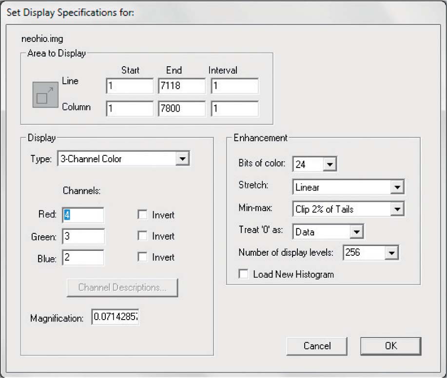
5. A new dialog box will appear to let you set the display specification for the ‘neohio’ image.
   

   (Source: Purdue Research Foundation)
6. Under Channels, you will see the three color guns available to you (red, green, and blue). Each color gun can hold one band (see the Lab Data section for information on which bands correspond to which parts of the electromagnetic spectrum). The number listed next to each color gun represents the band being displayed with that gun.
7. Display band 4 in the red color gun, band 3 in the green color gun, and band 2 in the blue color gun.
8. Accept the other defaults for now and click OK.
9. A new window will appear, and the ‘neohio’ image will load in it.

11.2 Subsetting Images and Examining Landsat Imagery

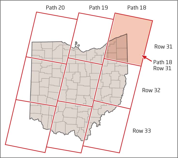
Right now, you’re working with an entire Landsat TM scene, which is an area roughly 170 kilometers long by 183 kilometers wide (as shown in the graphic below—you are using the scene encompassed by path 18, row 31). For this lab, we want to focus only on the area surrounding downtown Cleveland. You will have to create a subset—in essence, “clipping” out the area that you’re interested in, and creating a new image from that.

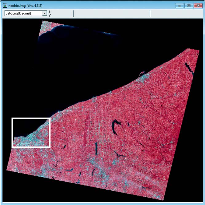
1. Zoom to the part of the ‘neohio’ image that shows Cleveland (as in the graphic below):
   

   (Source: Purdue Research Foundation)
2. In the image, you should be able to see many features that make up downtown Cleveland—the waterfront area, a lot of urban development, major roads, and water features.
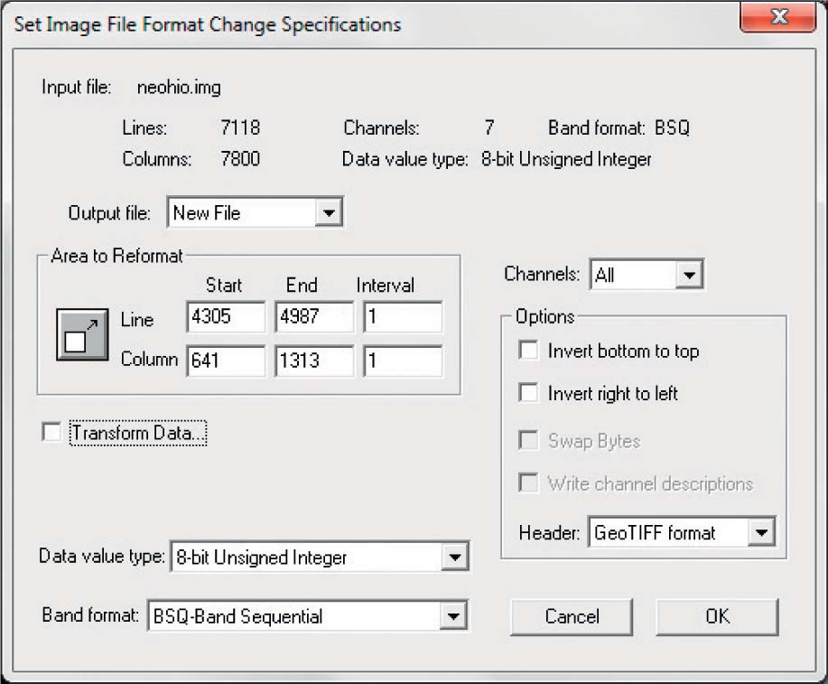
3. In order to create a new image that shows only Cleveland (a suggested region is shown in the graphic above), select Reformat from the Processor pull-down menu, then select Change Image File Format.
4. You can draw a box around the area you want to subset using the cursor, and the new image that’s created will have the boundaries of the box you’ve drawn on the screen. However, for the sake of consistency in this exercise, use the following values for the Area to Reformat:
   1. Line:
      • Start 4305
      • End 4987
      • Interval 1
   2. Column:
      • Start 641
      • End 1313
      • Interval 1
   
   Leave the other defaults alone and click OK.
   
   

   (Source: Purdue Research Foundation)
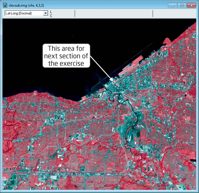
5. In the Save As dialog box that appears, save this new image in the Chapter11 folder (call it clevsub.img). Choose Multispectral for the Save as Type option (from the pull-down menu options next to Save as Type). When you’re ready, click Save.
6. Back in MultiSpec, minimize the window containing the ‘neohio’ image.
7. Open the clevsub image you just created in a new window (in the Open dialog box, you may have to change the Files of Type that it’s asking about to “All Files” to be able to select the ‘clevsub’ image option).
8. Open the clevsub image with a 4-3-2 combination (band 4 in the red gun, band 3 in the green gun, and band 2 in the blue gun).
9. Use the other defaults for the Enhancement options (stretch is Linear and range is Clip 2% of tails).
10. In the Set Histogram Specifications dialog box that opens, select the Compute new histogram method, and use the default Area to Histogram settings.
11. Click OK when you’re ready. The new subset image shows that the Cleveland area is ready to use.
12. Zoom in on the downtown Cleveland area, especially the areas along the waterfront. Answer Questions 11.1 and 11.2. (You will want to also open Google Earth and compare the Landsat image to its very crisp resolution imagery when you answer these questions.)

11.3 Examining Landsat Bands and Band Combinations

1. Zoom in on the waterfront area, looking at FirstEnergy Stadium, home to the Cleveland Browns, and its immediate surrounding area.
   

   (Source: Purdue Research Foundation)
2. Open another version of the ‘clevsub’ image using the 3-2-1 combination.
3. Arrange the two windows on the screen so that you can examine them together, expanding and zooming in as needed to be able to view the stadium in both three-band combinations.

   Question 11.3

   Which one of the two-band combinations best brought the stadium and its field to prominence?

   Question 11.4

   Why did the band combination you chose best help in viewing the stadium and the field? (Hint: You may want to do some brief online research into the nature of the new stadium and its field.)
4. Return to the view of Cleveland’s waterfront area. You’ll now be examining the water features (particularly Lake Erie and the river). Paying careful attention to the water features, open four display windows, then expand and arrange them side by side to look at differences between them. Create the following image composites (one for each window):
   1. 3,2,1
   2. 7,5,4
   3. 4,2,1
   4. 1,1,1

   Question 11.5

   Which band combination(s) is best for letting you separate water bodies from land? Why?
5. Return to the view of Cleveland’s waterfront area. Focus on the urban features and vegetated features (zoom and pan where necessary to get a good look at urbanization). Open new windows with some new band combinations, and note how things change with each one as follows:
   1. 7,4,2
   2. 1,2,3
   3. 4,3,2

   Question 11.6

   Which band combination(s) is best for letting you separate urban areas from other forms of land cover (that is, vegetation, trees, etc.)? Why?
6. Open a new display window and examine the full view of the entire ‘clevsub’ image. Open this window with the following band combination:
   1. 6,6,6
7. Zoom in and move around the Cleveland waterfront area that we’ve been examining.

   Question 11.7

   Why is the image so “blurry” or “fuzzy” in this combination (compared to all the other band combinations you’ve looked at in this exercise)?

Closing Time

This exercise wraps up working with Landsat information as well as working with imagery in MultiSpec. Chapter 12 focuses on a whole different set of remote sensing satellites (part of the Earth Observing System), and its exercise will return to Google Earth to examine this imagery.

Exit MultiSpec by selecting Exit from the File pull-down menu. There’s no need to save any work in this exercise.