12.1 Geospatial Lab Application: Earth Observing System Imagery

This chapter’s lab will introduce you to some of the basics of examining EOS (Earth Observing System) imagery from the Terra and Aqua satellites. You will be examining data from MOPITT as well as many types of MODIS imagery, and you will be using online resources from NASA and others in conjunction with Google Earth.

Objectives

The goals of this lab are:

• to examine the usage and function of MODIS imagery.
• to utilize Google Earth as a tool for examining remotely sensed EOS imagery.
• to use Terra and Aqua imagery for environmental analysis.

Obtaining Software

The current version of Google Earth (7.1) is available for free download at http://earth.google.com.

Important note: Software and online resources sometimes change fast. This lab was designed with the most recently available version of the software at the time of writing. However, if the software or Websites have significantly changed between then and now, an updated version of this lab (using the newest versions) is available online at http://www.whfreeman.com/shellito2e.

Using Geospatial Technologies

The concepts you’ll be working with in this lab are used in a variety of real-world applications, including:

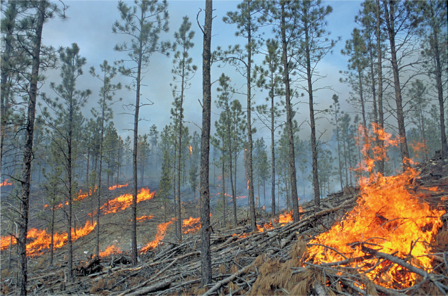
• forestry—MODIS imagery can be accessed by forest rangers on a near-daily basis to aid in active wildfire and forest fire monitoring.
• climatology—MODIS imagery can be used to track and monitor hurricanes and tropical storms, and this information in turn is of help to emergency preparedness programs.

(Source: © Karen Wattenmaker/www.forestphoto.com)

Lab Data

Copy the folder Chapter12—it contains the following KML datasets (for Google Earth) from NASA’s Earth Observatory:

• russia_tmo_2012170.kml—this MODIS image shows fires in Siberia.
• ge_44478.kml—this MODIS image shows a phytoplankton bloom off the coast of Iceland.
• irene_amo_2011238.kml—this MODIS image shows Hurricane Irene.
• isaac_tmo_2012241.kml—this MODIS image shows Hurricane Isaac.

Chapter12 also contains the following KML datasets from NASA/Goddard Space Flight Center and NASA’s Scientific Visualization Studio:

• a002900.kml – this is an animation of MOPITT imagery from Terra
• a003255.kml – this is an animation of MODIS imagery from Aqua

Localizing This Lab

This lab uses EOS data from a variety of locations across the globe, but there are several ways to examine some EOS imagery at a more local level:

In Section 12.1, take a look through the NASA Earth Observatory Website and archived information, and look for some related phenomena (such as other fires or storms) that are either relatively close to your location or whose MODIS imagery overlaps into your area.

In Section 12.2, examine one year’s worth of MOPITT data to determine conditions in your local area, rather than on a global scale, and keep track of the carbon monoxide (CO) levels for your region.

In Sections 12.3 and 12.4, examine some of the Terra and Aqua imagery products to determine the climatic interactions in your region, rather than on a global scale. Open and examine images from multiple dates in Google Earth for your area, rather than one month’s worth of data.

12.1 Viewing MODIS Imagery with Google Earth

1. Start Google Earth.
2. We’ll begin by examining a MODIS image of wildfires burning in Siberia. More information about this is available through NASA’s Earth Observatory here: http://earthobservatory.nasa.gov/IOTD/view.php?id=78305. The MODIS image comes in a format called KML which can be read by Google Earth and overlaid on top of the normal Google Earth imagery. From the File pull-down menu, select Open. Navigate to the Chapter 12 folder, select the russia_tmo_2012170.kml file, and click Open. A new item called “Siberia Burns” will be added to Google Earth’s Temporary Places, and the view will rotate to the location of the image. Note that you can turn the image display on and off by clicking a checkmark in the “Siberia Burns” box.
3. Owing to the large extent of the MODIS image, you’ll have to zoom out to see the whole thing, but then zoom in to different parts of it to examine the fires themselves.

   Question 12.1

   WVP7u7sqlmhY+Qp+njG2bUrNJt14+Rxr//ZUadI38/65HujokJptkIii5Cz6IPVQnYyOyZxxJ/s=

   Question 12.2

   1rvIna+biYM1mYQlD78Q6aExCP6yOc+e3ZY/aQawi0H6IE49981f45uyhJ+RmPAXL3l1gOnf/PFQodoMwgC5pLlyXnj8rca9/8htGGNCk0BQps4BuRspeSiYBqFWFrJwhB40T97vKnv15UJNC4YMkfNP/8zLhR6UxslQ8YqaeVwO5nfvqri8ulYJXO4=
4. Next, we’ll examine a MODIS image of a phytoplankton bloom off the coast of Iceland. More information about this is available through NASA’s Earth Observatory here: http://earthobservatory.nasa.gov/IOTD/view.php?id=44478. Open a new KML file, the one called ge_44478.kml. Google Earth will rotate around to Iceland, and a new MODIS scene will appear (and a new item called “Phytoplankton Bloom off Iceland” will be added to your Temporary Places).
5. Again, you may have to first zoom out to see the extent of the MODIS image and then zoom in to examine some of the details.
   

   Question 12.3

   Dm/6w+a8hKeqNEDg+OKkF2fRM3pUnzdWWi1VT2TDhERIICdMmPEIWdfXsv5LPOMVqGRvZik8sJ3u0jUGU7YBhdgM9KO1/Opw5LJX3+C3/v2eHXG1K6RA2G8ZjB+oKoRVRtVn/MUcNeeRaJFuO30/UZfDRNnnfO9CjnbBBoBGgod7x17e2CpfzVX9ErRvI+wj6rzTcZe1GaPx4YQHQW0pqTrW6wXsW2Tf3ZRb4yP5lPHzv5P1nGjQnyNaOnLD9MEDVHqOc0zoSJ2kQdO5bTP+vvexHpy6ZdkrpG1/vn0GS5rbDwd7fbtd8DV8yIkJ2DkC3UCOLg==
6. Lastly, we’ll be examining MODIS imagery of large destructive storms, particularly Hurricane Irene from 2011 and Hurricane Isaac from 2012. More information about monitoring these two storms is available here: for Irene, at http://earthobservatory.nasa.gov/NaturalHazards/view.php?id=51931; and for Isaac, at http://earthobservatory.nasa.gov/IOTD/view.php?id=79008. Open a new KML file called irene_amo_2011238.kml to view the MODIS imagery of Hurricane Irene. Google Earth will rotate to the east coast of the United States. As with the other MODIS images, you’ll have to zoom out to see the extent of the imagery of Irene.
7. Once you’ve examined the MODIS image of Irene, open a new KML file called isaac_tmo_2012241.kml, which is of Hurricane Isaac. Zoom out from the image. You’ll see the two hurricane images overlap, so you’ll have to turn one image off and the other on to examine both of them.
   

   Question 12.4

   8wGTHZjig/othnNFl4+GrDQdGqJ1nB3XdpQa7zUO1jEMuI3De0V0FmasEDZY0zMzOsUe+7IFBze8ZW5+BEBDbjLgnhOJWeK+NV5FPWc+99oDlyeLg9WzdVgpcd2EwkhwjMKOK/CqYvZqHE31oC/rAFUJ9AzAvDzBV0eAj5THBWwgRidfPy2YdnqOYK/wWm+iFf0aLjxuhgl1hQjIYHCrlnw+vGQ=
8. At this point you can turn off all four of your KML files.

12.2 Using NASA Scientific Visualization Studio Imagery in Google Earth

Data from NASA’s Scientific Visualization Studio (SVS) provides imagery or animations pertaining to several dates, and these images are placed together as a time series. Some of these animations have been formatted to work with Google Earth as KML files.

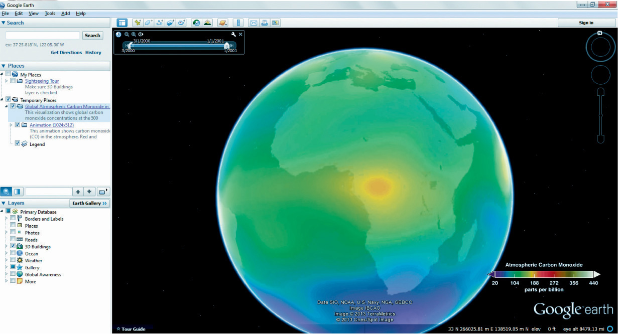
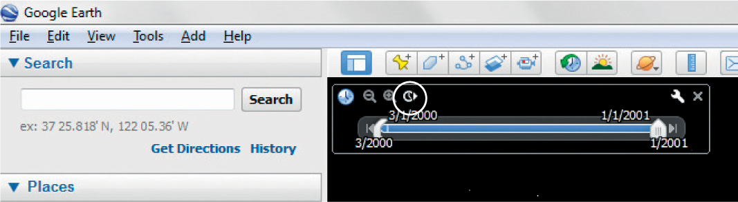
1. Open a new KML file called a002900.kml. A new item will be added to Google Earth’s Temporary Places called “Global Atmospheric Carbon Monoxide in 2000,” which is a series of MOPITT images from March through December 2000. More information about this can be found at the SVS Website at: http://svs.gsfc.nasa.gov/vis/a000000/a002900/a002900. You’ll see that a legend has been added to Google Earth as well, showing which colors on the image correspond to what levels of carbon monoxide. If necessary, use the Google Earth tools to adjust the view so that all of Earth is shown in the Viewer.
   
   

   (Source: Google)
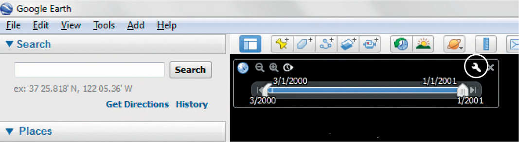
2. A slider bar has also been added to the top of the Google Earth display. You can use this slider bar to step through the MOPITT imagery day by day.
3. To animate the data, click on the wrench icon on the slider bar.
   
   

   (Source: Google)
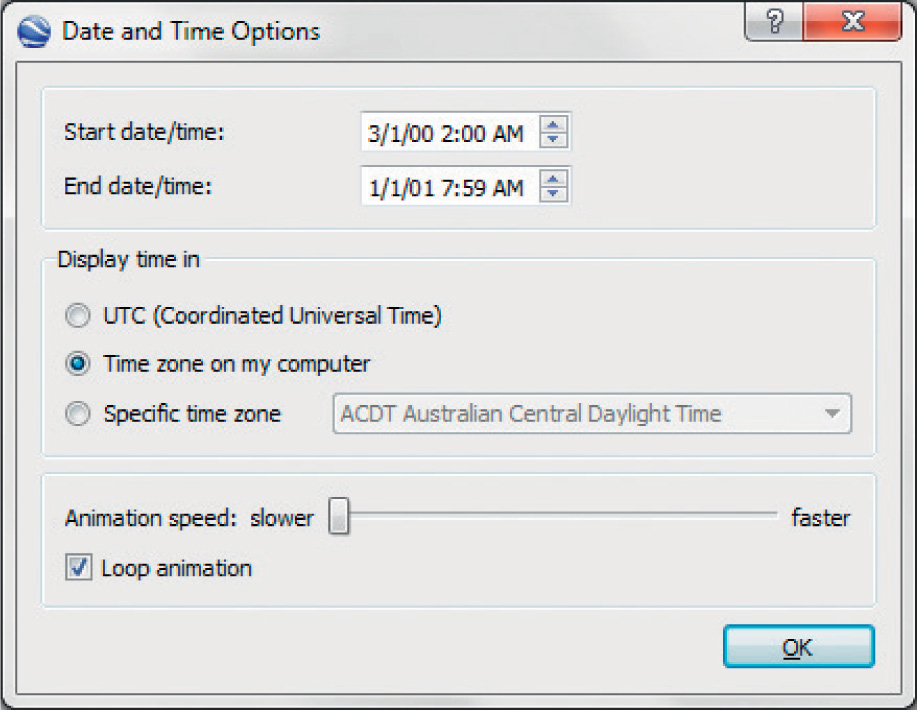
4. In the Date and Time Options box that opens, select March 1, 2000, as the Start date/time and January 1, 2001, as the End date/time.
5. Reduce the Animation speed slider from fastest back to the slowest option on the left.
   
   

   (Source: Google)
6. Place a checkmark in the Loop animation box. Click OK to close the dialog.
   
   

   (Source: Google)
7. Click on the Play animation button on the slider bar to begin the animation.
8. Some frames might come up blank or the animation may not play at first—Google Earth seems to need to run completely through the animation once for it to load all the MOPITT imagery. On the second run-through of the animation, there should be no blank spots in the data.
9. You can press the Play animation button (it will now have a pause symbol) at any time to stop the animation from playing. Answer Questions 12.5 and 12.6. (You will have to rotate the globe while the animation is playing to answer the questions—also keep in mind the times and dates that are running in the upper-right-hand side of the screen. You may want to pause or rewind to examine certain dates in the past.)
   

   Question 12.5

   aYCI61bZDTNRK+B9qx7U4jdhyBlBw//hxu39uUrSBxOXZzUFwm2HwElgu/PN/ypJMAs5JCfuy7xBBSTv4KYFJbJabmDPDU9hWjwC1+JWRrMFspQ8lCywnk1fHa1qDWu6VljHCaAYfp/9XvOBQBa9Y0YI+lOwMUIVAlazXw==

   Question 12.6

   in3lvR6Ai/a0qNlssAZB7osPJdaQlt/L/O+nkgRpTNUGdjcTNLogtY1V5k0MpukbiaK7jNChTfq82TMO6W/MMUUTH2G/7j6We1+AoWEfuTAagtRhjgaDNPxQ3tJsukAOK6Xb6ZJlfx5fjr/1loqht6nsgbj5cjKhRSFnBdz345AhqVVjZnNDSVYzWS7GMWcL1qzfa7uDz7ft70adNbmPD3ZoIVh06Yu7UpylsFs3oRTZw/ru3LXCqDh63cwJ2l1FTCz6QiC3+5+3xiATYqiJrPO1BBPFJ1BN9ZmsAQ==
10. Turn off the Global Atmospheric Carbon Monoxide in 2000 KML file when you’re done.
11. Next, open another Scientific Visualization Studio KML called a003255.kml. A new item will be added to Google Earth’s Temporary Places called “Aqua MODISimagery of Hurricane Katrina,” and Google Earth will rotate to the Gulf Coast of the United States. More information about this MODIS imagery this can be found here: http://svs.gsfc.nasa.gov/vis/a000000/a003200/a003255.
12. Set up the animation as you did with the MOPITT carbon monoxide animation, and play this new animation. It will show several days of imagery from the MODIS instrument on Aqua, during which time Hurricane Katrina was building before making landfall on the Mississippi Gulf Coast. You may have to pause or replay the animation to view all of the imagery.
    

    Question 12.7

    MvycugSjt+P03P92KJ9ByJDyFRMFDOxZInyBdA3oLG1FlNMLftSj3fUucOxMLSvTUBRFkfvgaglygIiymGowmUH70yF46ApL3CZQ5qxu1AMglJ7GIXlLHz8e1gQX0/bn/wyp3KOkPUuH0RByidODV6L/yvOjPyqR106QgPe0Oj/2t00z9acKTNx9q1Pi9AbFCgGa94J1S9zvq4vyvD8f8noHZnepPOYOedU00rQnWLUXJL67ZICBRcpjKSgKDcuo4SPX9wdh25lgcxQ60qg1HQ==
13. Turn off the Aqua MODIS imagery of Hurricane Katrina when you’re done.

12.3 Using the NASA Earth Observations (NEO) Web Resources

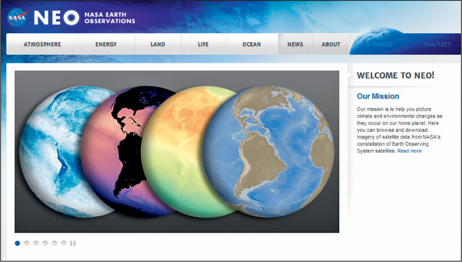
1. Open your Web browser and go to http://neo.sci.gsfc.nasa.gov. This is the Website for NEO (NASA Earth Observations), an online source of downloadable Earth observation satellite imagery. In this portion of the lab, you’ll be using NEO’s EOS imagery in conjunction with Google Earth in a KMZ format (which is a compressed version of KML).
   
   

   (Source: NASA)
2. Click on the Atmosphere option at the top of the page.
3. Select the option for Carbon Monoxide.
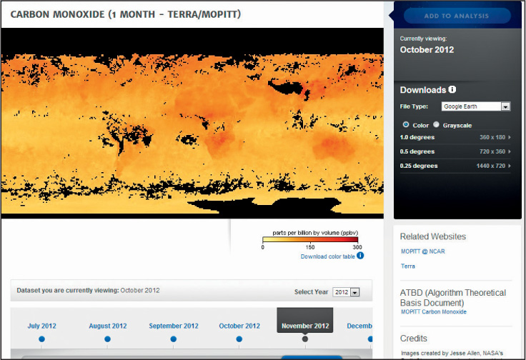
4. This is an image of global carbon monoxide concentration for one month, collected using the MOPITT instrument aboard Terra (see the section on About this dataset for more detailed information).
5. Rather than providing you with a view of a flat satellite image, NEO gives you the option of examining the imagery draped across a virtual globe.
6. Select 2012 for the year and then choose the option for November 2012 (this will display imagery from October 2012, which is what we want to examine). From the Downloads pull-down menu select Google Earth, then click on the option for 1440 × 720 to begin the download of the KMZ file. Locate the downloaded KMZ file on your computer and double-click it to open the file in Google Earth.
   
   

   (Source: NASA Earth Observations (NEO))
7. Rotate Google Earth to examine the MOPITT imagery draped over the globe.
   

   Question 12.8

   ckyAkhBzQd9zx4lS3CryZHJoSuLTNgGDpdYmnNkAnLoMX6yj7+VNcW+62d0nTiZY2gMIU3+X8plTMgZbsh8FgcxAMDTpURakFm+E/sPZps6u64q+whJogBN/Ev/7Oxzk
8. Back on the NEO Website, select the Energy tab, then select Land/Surface Temperature [Day].
9. Choose the option for 2012, then select October (to view September imagery).
10. Use Google Earth for the Downloads option and click on the 1440 × 720 option.
11. In Google Earth, turn off the MOPITT image (it will be in your Temporary Places listings).
    
    

    (Source: Google)
12. Rotate Google Earth to examine the new MODIS image.
    

    Question 12.9

    WKb4BnBx4mRbnhLRDcIRhmtEMVvrfxsit9rDMydggCChCa303ag/j5hhwfBiaHFEUyCaQtkhsRgY+K5MXJvASwpRXjSkenr1IpZw++8ujWzJu3RlMRuS+A==
13. Back on the NEO Website, select the Life tab, and then select Vegetation Index [NDVI]. Choose the image for 2012, then select August (to view the July imagery).
14. NDVI is a metric used for measuring vegetation health for a pixel. As we discussed in Chapter 10, the higher the value of NDVI, the healthier the vegetation at that location.
15. Use Google Earth for the Downloads option and click on the 1440 × 720 option.
16. In Google Earth, turn off your other two Terra images.
17. Rotate Google Earth and zoom in to examine the new MODIS composite image.
    

    Question 12.10

    w+oXorPgRVmuKJkW4Mk54FdsEAet+Vp4lF7DgrFJo1F10IRVCkAhEKfjVEOdsGOisrDiiGQsLnz0GETWfhY/UfyaGCoaPQEIMkQkpOivpTFx2AjfcbYsuj/vJsNArsvI/MlqvQaTfcDiDojcao6i2uI47vM=

12.4 EOS Imagery from the National Snow and Ice Data Center

1. NASA NEO is not the only source of EOS data for viewing in a virtual globe format. One example is the National Snow and Ice Data Center (NSIDC). Open your Web browser and go to their Website at http://nsidc.org/data/virtual_globes.
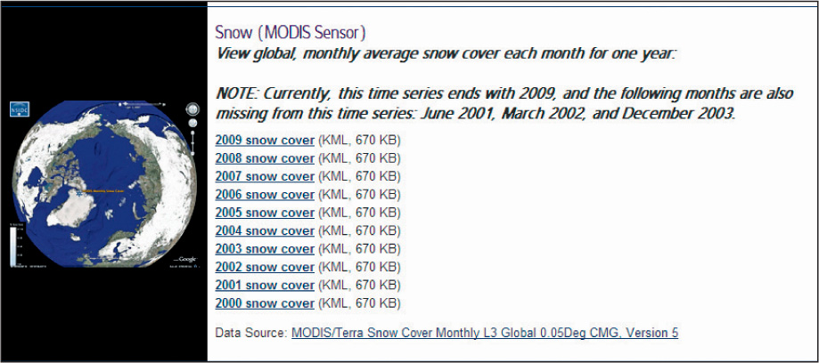
2. Go to the Featured Data section of the Website. Look for the section called Snow.
   
   

   (Source: National Snow and Ice Data Center (NSIDC)
3. Read about what the imagery is showing, and then open the KML file for 2009 snow cover. The KML file will open in Google Earth, like the ones from NEO.
4. In Google Earth, turn off your other three NEO images.
5. In Google Earth’s Temporary Places, there will be a new expandable item for NSIDC. By expanding this item and looking through the options, you’ll see another expandable item called Snow Cover. This shows that snow data for each month of 2009 is available as an option that can be clicked on and off. To examine just one month of data, turn off all of the other months. You can also use the slider bar that appears at the top of the Google Earth view to adjust the snow data in Google Earth from month to month.
6. Rotate Google Earth and zoom in to examine the new MODIS image.
   

   Question 12.11

   v8w9d75GoYYS2JXdO7YOaz87B9wZGBX8Mj+OSBsUR4EjvarSp+/MRNFpJlqKZQY2/dRIsqKPksWkk+bh0GHU8JHdX57b2SSco1NwCtePCrqKuEsnM43mHfIYNZC1ddIujNS9H/73FYdY87Fm915U/Ekok+s=

   Question 12.12

   MMJdpNa4J/jVnKAU8QdKcpNxuWsFAKOu0mfDXLKTsEt6rDdCgrmOsStlCpfR+H/NRR8M6NFgZ1FZUiODMwKklyWrENgsRY/oqW/UHxSZ6OFeJzisHI3XzM7bBwtCJ8jBYaZ3Dn7ysWx/qrBYr+ohxhT0hhjDFVRU
7. At this point, you can exit Google Earth by selecting Exit from the File pull-down menu and also close your Web browser.

Closing Time

This exercise showed off a number of different ways of viewing and visually analyzing data available from EOS satellites. The next chapter’s going to change gear, and we’ll start looking at the ground that those satellites are viewing.