6.2 
How Can You Perform Basic Spatial Analysis in GIS?
buffer a polygon of spatial proximity built around a feature
Once you have your selected data, it’s time to start doing something with it. A simple type of analysis is the construction of a buffer around the elements of a data layer. A buffer is an area of proximity set up around one or more objects. For instance, if you want to know how many rental properties are within a half-mile of a selected house, you can create a half-mile buffer around the object representing the house and then determine how many rental properties were within the buffer. Buffers can be created for multiple points, lines, or polygons (Figure 6.3). Buffers are simple tools to utilize, but they can provide useful information when you’re creating areas of analysis for various purposes.
dissolve the ability of the GIS to combine polygons with the same features together
GIS can also perform a dissolve operation, where boundaries between adjacent polygons that have the same properties are removed, merging the polygons into a single, larger shape. Dissolve is useful when you don’t need to examine each polygon, but only regions with similar properties. For example, suppose you have a land-use map of a county consisting of polygons representing each individual parcel and how it’s being used (commercial, residential, agricultural, etc.). Rather than having to examine each individual parcel, you could dissolve the boundaries between parcels and create regions of “residential” land use or “commercial” land use for ease of analysis. Similarly, if you have overlapping buffers generated from features, dissolve can be used to combine buffer zones together. See Figure 6.4 for an example of dissolve in action.
164
geoprocessing the term that describes when an action is taken to a dataset that results in a new dataset being created
Buffers and querying are basic types of spatial analysis, but they only involve a single layer of data (such as creating a buffer around roads or selecting all records that represent a highway). If you’re going to do spatial analysis along the lines of John Snow’s hunt for a cholera source, you’ll have to be able to do more than just select a subset of the population who died, or just select the locations of wells within the area affected by the disease—you’ll have to know something about how these two things interacted with each other over a distance. For instance, you’ll want to know something about how many cholera deaths were found within a certain distance of each well. Thus, you won’t just want to create a buffer around one layer (the wells)—you’ll want to know something about how many features from a different layer (the death locations) are in that buffer. Many types of GIS analysis involve combining the features from multiple layers together to allow examination of several characteristics at once. In GIS, when one layer has some sort of action performed to it and the result is a new layer, this process is referred to as geoprocessing. There are numerous types of geoprocessing methods, and they are frequently performed in a series to solve a spatial analysis question.
165
spatial query selecting records or objects from one layer based upon their spatial relationships with other layers (rather than using attributes)
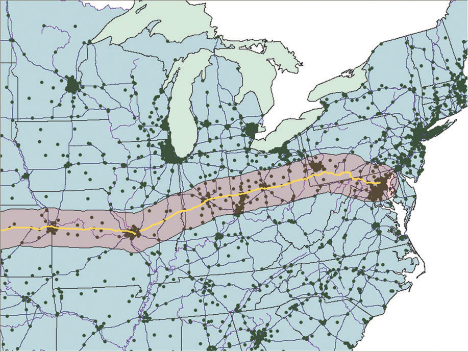
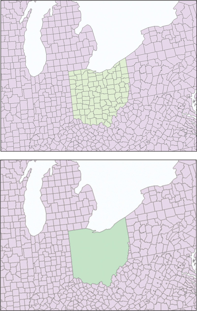
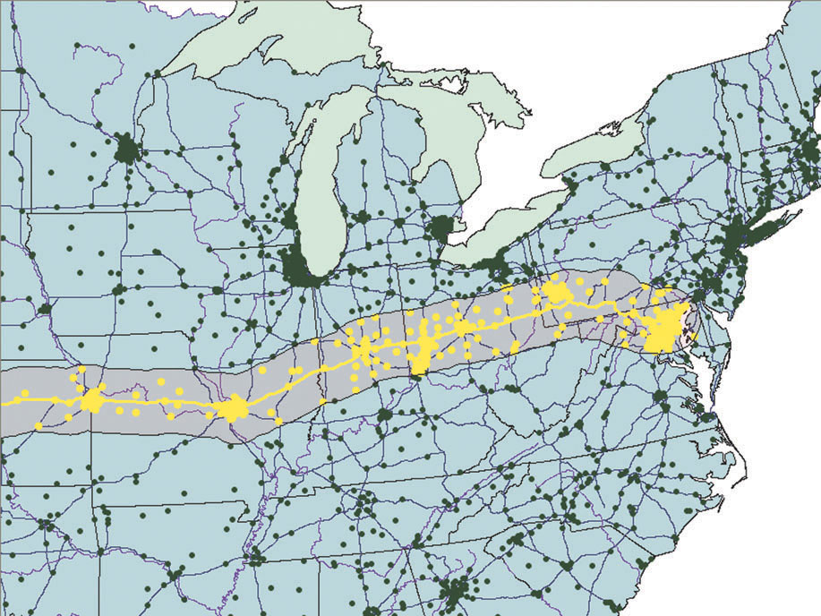
GIS gives you the ability not just to perform a regular SQL-style query, but to also perform a spatial query—to select records or objects from one layer based upon their spatial relationships with other layers (rather than using attributes). With GIS, queries can be based on spatial concepts—to determine things like how many registered sex offenders reside within a certain distance from a school, or which hospitals are within a particular distance of your home. The same kind of query would be done if a researcher wanted to determine which cholera deaths are within a buffer zone around a well. In these cases, the spatial dimensions of the buffer are being used as the selection criteria—all objects within the buffer are what will be selected. See Figure 6.5 for an example of using a buffer as a selection tool, as well as Hands-on Application 6.2: Working with Buffers in GIS.
166
 HANDS-ON APPLICATION 6.2
Working with Buffers in GIS
Honolulu has an online GIS application that looks at parcels and zoning for the area. On this Website, you can select a location, generate a buffer around it, and all parcels touched by the buffer can be selected (and their parcel records displayed). To use this, open your Web browser and go to http://gis.hicentral.com/fastmaps/parcelzoning—then zoom in to a developed or residential area (if you’re familiar with the area, you can also search by address). To generate a buffer, select the Tools icon, and then choose the option for Circle-Select Parcels. At this point, you can specify a buffer distance (the radius of the circle) and click on a place on the map. A buffer will be generated around your placemark, and the parcels selected by the buffer will be highlighted on the map and their records returned. Try examining some areas with various buffer sizes to see how buffers can be used as a selection tool.
Expansion Questions:

Question
Use the Search function and the Places of Interest option to locate “State Capital.” How many land parcels are within a 500-foot radius of a point placed at the center of the building?
-
Question
How many land parcels are within a 1000-foot radius of the same point?
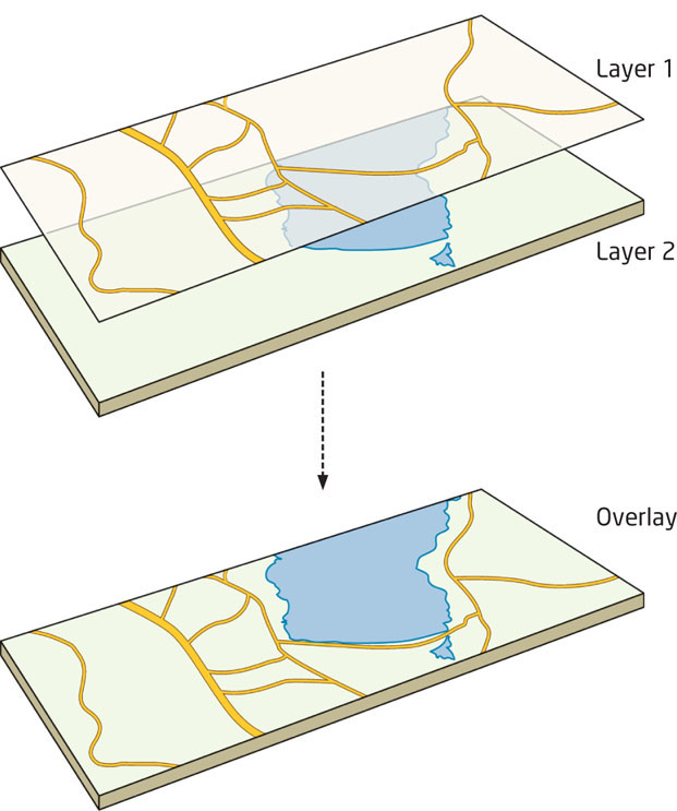
overlay the combining of two or more layers in the GIS
Other analyses can be done beyond selecting with a buffer or selecting by location. When two or more layers share some of the same spatial boundaries (but have different properties) and are combined together, this is referred to as an overlay operation in the GIS. For instance, if one layer contains information about the locations of property boundaries and a second layer contains information about water resources, combining these two layers in an overlay can help determine which resources are located on whose property. An overlay is a frequently used GIS technique for combining multiple layers together for performing spatial analysis (Figure 6.6).
intersect a type of GIS overlay that retains the features that are common to two layers
identity a type of GIS overlay that retains all features from the first layer along with the features it has in common with a second layer
symmetrical difference a type of GIS overlay that retains all features from both layers except for the features that they have in common
union (overlay) a type of GIS overlay that combines all features from both layers
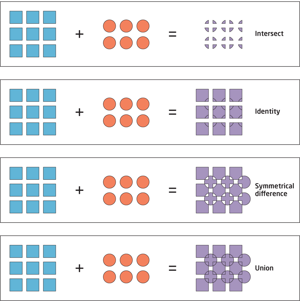
There are numerous ways that polygon layers can be combined together through an overlay in GIS. Here are some widely-used overlay methods Figure 6.7):
- Intersect: In this operation, only the features that both layers have in common are retained in a new layer. This type of operation is commonly used when you want to determine an area that meets two criteria—for instance, a location needs to be found within a buffer and also on a plot of land used for agriculture: you would intersect the buffer layer and the agricultural layer together to find what areas, spatially, they have in common.
- Identity: In this operation, all of the features of an input layer are retained, and all the features of a second layer that intersect with them are also retained. For example, you may want to examine all of the nearby floodplain and also what portions of your property are on it.
- Symmetrical difference: In this operation, all of the features of both layers are retained—except for the areas that they have in common. This operation could show you, for example, all potential nesting areas along with the local plan for development, except where they overlap (so those areas can be taken out of the analysis).
- Union (overlay): In this operation, all of the features from both layers are combined together into a new layer. This operation is often used to merge features from two layers (for instance, in order to evaluate all possible options for a development site, you may want to overlay the parcel layer and the water resources layer together).
map algebra combining datasets together using simple mathematical operators
Another way of performing spatial overlay is by using raster data. With raster cells, each cell has a single value, and two grid layers can be overlaid in a variety of ways. The first of these is by using a simple mathematical operator (sometimes referred to as map algebra), such as addition or multiplication. To simplify things, we’re only going to assign our grids values of 0 or 1, where a value of 1 means that the desired criteria are met and a value of 0 is used when the desired criteria are not met. Thus, grids could be designed using this system with values of 0 or 1 to reflect whether a grid cell meets or does not meet particular criteria.
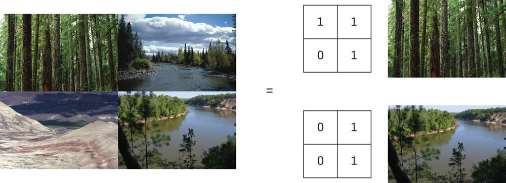
Let’s start with a simplified example—say you’re looking to find a plot of land to build a vacation home on, and your two key criteria are that it be close to forested terrain for hiking and close to a river or lake for water recreation. What you could do is get a grid of the local land cover and assign all grid cells that have forests on the landscape a value of 1 and all non-forested areas a value of 0. The same holds true for a grid of water resources—any cells near a body of water get a value of 1 and all other cells get a 0. The “forests” grid has values of 1 where there are forests and values of 0 for non-forested regions, while the “water” grid has values of 1 where a body of water is present and values of 0 for areas without bodies of water (see Figure 6.8 for a simplified way of setting this up).
168
169
Now you want to overlay your two grids and find what areas meet the two criteria for your vacation home, but there are two ways of combining these grids. Figure 6.9 shows how the grids can be added and multiplied together with varying results. By multiplying grids containing values of 0 and 1 together, only values of 0 or 1 can be generated in the resulting overlay grid. In this output, values of 1 indicate where (spatially) both criteria (forests and rivers) can be found, while values of 0 indicate where both cannot be found. In the multiplication example, a value of 0 could have one of the criteria, or none, but we’re only concerned with areas that meet both criteria, or else we’re not interested. Thus, the results either match what we’re looking for or they don’t.
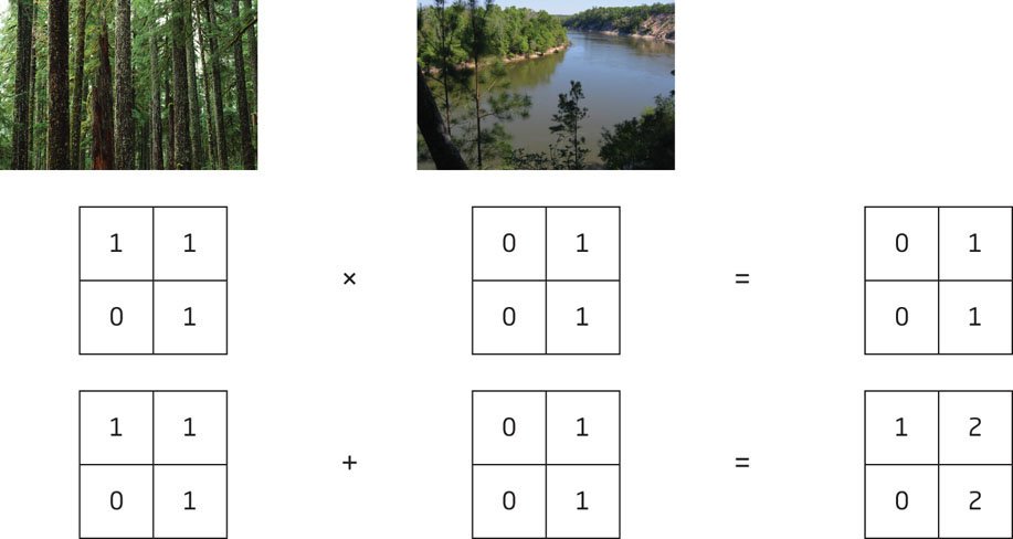
In the addition example, values of 0, 1, or 2 are generated from the overlay. In this case, values of 0 contain no forests or rivers, values of 1 contain one or the other, and values of 2 contain both. By using addition to overlay the grids, a gradient of choices is presented—the ideal location would have a value of 2, but values of 1 represent possible second-choice alternatives, and values of 0 represent unacceptable locations.
site suitability the determination of the “useful” or “non-useful” locations based on a set of criteria
This type of overlay analysis is referred to as site suitability, as it seeks to determine which locations are the “best” (or most “suitable”) for meeting certain criteria. Site suitability analysis can be used for a variety of topics, including identifying ideal animal habitats, prime locations for urban developments, or prime crop locations. When using the multiplication operation, you will be left with sites classified as “suitable” (values of 1) or “non-suitable” (values of 0). However, the addition operation leaves other options that may be viable in case the most suitable sites are unavailable, in essence providing a ranking of suitable sites. For instance, the best place to build the vacation home is in the location with values of 2 since it meets both criteria, but the cells with a value of 1 provide less suitable locations (as they only meet one of the criteria).
170