6.1 Geospatial Lab Application: GIS Spatial Analysis: QGIS Version

This chapter’s lab builds on the basic concepts of GIS from Chapter 5 by applying several analytical concepts to the GIS data that you used in that chapter’s labs. This lab also expands on Chapter 5 by introducing several more GIS tools and features, and explaining how they are used.

Similar to the two Chapter 5 geospatial lab applications, two versions of this lab are also provided. The first version (Geospatial Lab Application 6.1: GIS Spatial Analysis: QGIS Version) uses the free QGIS package. The second version (Geospatial Lab Application 6.2: GIS Spatial Analysis: ArcGIS Version) provides the same activities for use with ArcGIS 10.1 or 10.2. Although ArcGIS contains more functions than QGIS, these two programs share several useful spatial analysis tools.

Objectives

The goals for you to aim for in this lab are:

• to construct database queries in QGIS.
• to create and use buffers around points, lines, and polygons.
• to use different selection criteria (from queries) to perform simple spatial analysis.

Obtaining Software

The version of QGIS used in this lab is 1.8.0, and available for free download at: http://qgis.org/downloads.

Important note: Software and online resources sometimes change fast. This lab was designed with the most recently available version of the software at the time of writing. However, if the software or Websites have significantly changed between then and now, an updated version of this lab (using the newest versions) is available online at http://www.whfreeman.com/shellito2e.

Using Geospatial Technologies

The concepts you’ll be working with in this lab are used in a variety of real-world applications, including:

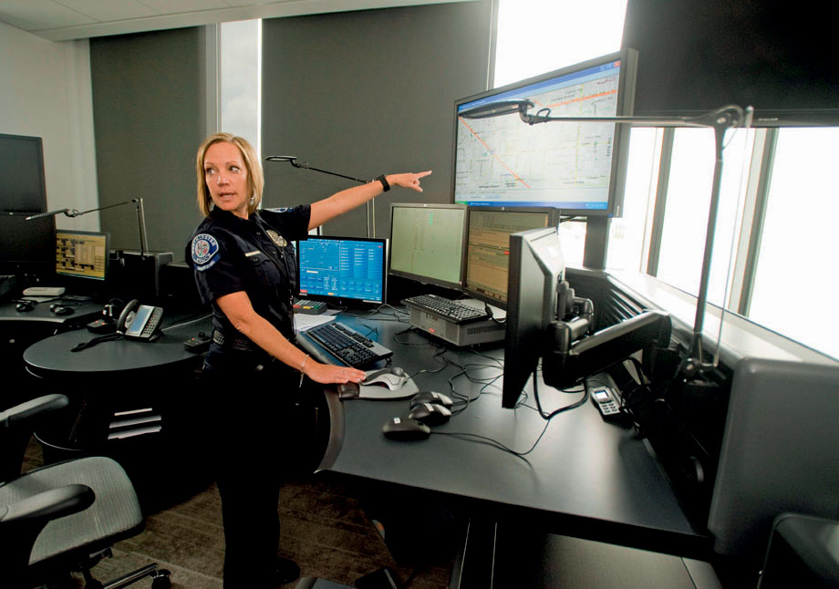
• law enforcement, where officers use spatial analysis techniques for examining “hot spots” of crimes as well as examining where different types of crimes are occurring in relation to other locations.
• emergency management services, which use spatial analysis for a variety of applications, such as researching what populated areas are covered (or not covered) by tornado sirens.

(Source: © ZUMA Press, Inc./Alamy)

Lab Data

Copy the folder Chapter6QGIS—it contains a folder called “usaproject,” in which you’ll find several shapefiles that you’ll be using in this lab. This data comes courtesy of Esri and was formerly distributed as part of their free educational GIS software package ArcExplorer Java Edition for Educators (AEJEE). For use in this lab with QGIS, it has already been projected for you to the US National Atlas Equal Area projection.

Localizing This Lab

The dataset used in this lab is Esri sample data for the entire United States. However, starting in Section 6.2, the lab focuses on North Dakota and South Dakota and the locations of some cities and roads in the area, and then switches to the Great Lakes region in Section 6.6. With the sample data covering the state boundaries and city locations for the whole United States, it’s easy enough to select your city (or cities nearby), as well as major roads or lakes, and perform the same measurements and analysis using those places more local to you than the ones in these areas.

6.1 Some Initial Pre-Analysis Steps

1. Start QGIS.
2. From the usaproject folder, add the following shapefiles: statesproject, citiesproject, lakesproject, riversproject, and intrstatproject.
3. Change the color schemes and symbology of each layer to make them distinctive from each other when you’ll be doing analysis. (See Geospatial Lab Application 5.1: GIS Introduction: QGIS Version for how to do this.)
4. Position the layers in the Map Legend so that all layers are visible (that is, the states layer is at the bottom of the Map Legend and the other layers are arranged on top of it).
5. When the layers are set how you’d like them, zoom in on South Dakota, so the state (and the nearby data) fills up the screen.

6.2 Database Queries

A database query is a standard feature in QGIS. We’ll start off with a simple query (using only one expression).

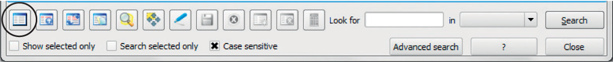
1. To build a query in QGIS, select the layer you want to query (in this case, citiesproject) by clicking on its name in the Map Legend. Then select the Open Attribute Table icon from the toolbar:
   

   (Source: QGIS)
2. The citiesproject attribute table will open as a new window. To query this layer, click on the Advanced search button at the bottom of the attribute table to open the query builder.
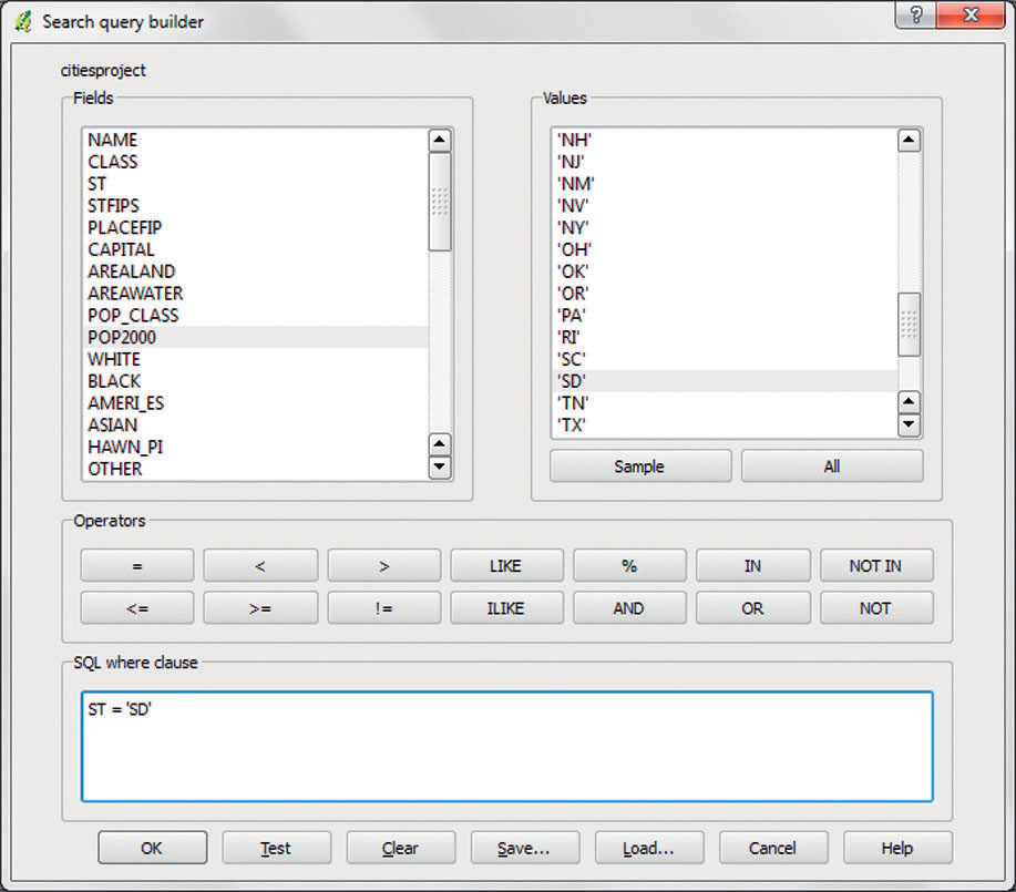
3. To build a query, first select the Field to use. In this case, double-click ST (which contains the state name abbreviations).
4. Next, select an Operator to use. In this case, select the = operator.
5. Lastly, select the appropriate Values. Click on the All button to show a list of all available values for the Field called ST. For this query, double-click the Value called ‘SD’ (which stands for South Dakota). The query will appear in the SQL where clause box as: ST = ‘SD’. This will select all records whose ST field are equal to the characters ‘SD’.

   180

   

   (Source: QGIS)
6. Click OK to run the query. After it runs, the query builder will close and you’ll return to the attribute table. The number of returned records will be shown at the top of the attribute table dialog box—you’ll see that this particular query will return nine records. To see which records (i.e., cities) these are, place a checkmark in the Show selected box at the bottom of the attribute table.
7. Take a look at the Map View again and you’ll see that those nine cities in South Dakota have turned yellow (and have been selected).
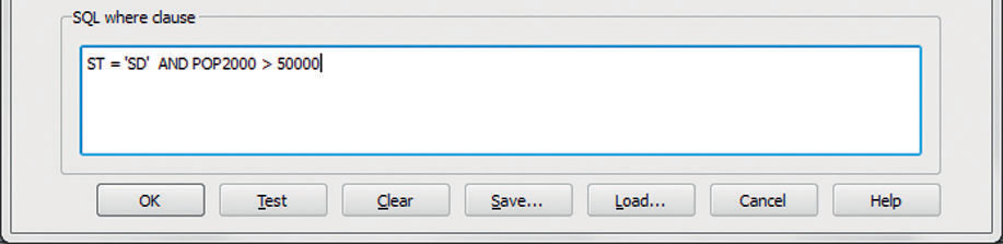
8. Next, we’ll build a compound query to find all of the cities in South Dakota with a Year 2000 population of greater than 50,000 persons. Bring up the query builder again, this time creating a query looking for ST = ‘SD’ (but don’t click OK yet).
9. Now click the button for the AND operator, then finish the second half of the compound query by selecting POP2000 as the Field, then select the greater than Operator (>), and lastly, type in the number 50000 in the SQL where clause box. Your final query should look something like this:

   181

   

   (Source: QGIS)
10. Click OK to query the database.

6.3 Creating and Using Buffers around Points

1. QGIS allows you to create buffers around objects for examination of spatial proximity, and gives you the ability to use the spatial dimensions of the buffer as a means of selecting other objects.
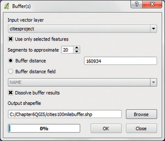
2. To create a buffer, first select the layer whose selected features you wish to buffer from the Map Legend (in this case, select the citiesproject layer).
3. Next, from the Vector pull-down menu, select Geoprocessing Tools, then select Buffer(s).
4. The Buffer dialog box will appear:
   

   (Source: QGIS)
5. We’ll start with a simple buffer around the cities, so the Input vector layer should be citiesproject.
6. Place a checkmark in the box next to Use only selected features. This will create a buffer around the cities you selected for Question 6.1.
7. Set the Segments to approximate option to 20. This is a measure of the “smoothness” of the buffer being created by QGIS.
8. Select the ratio button next to Buffer distance and type in 160934. This value is the number of meters equal to 100 miles. Since your citiesproject data is being measured in meters, QGIS will use that for the buffer’s units of measurement.
9. Place a checkmark in the box next to Dissolve buffer results.
10. Click the Browse button and navigate to your C:\Chapter6QGIS folder. Name the Output shapefile (the buffer that will be created) cities100milebuffer.shp and Save it.
11. Back in the Buffer(s) dialog box, click OK to create the buffer.
12. When prompted about adding the new layers to the Map Legend, click Yes. The circular 100-mile buffers will be created around the selected cities. Close the Buffer(s) dialog, then drag your citiesproject layer to the top of the layers in the Map Legend.
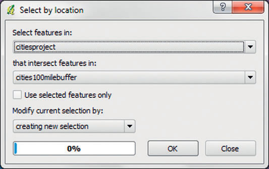
13. QGIS allows you to select features based on their proximity to other features. For instance, you can find out how many cities are within the buffer you just created and create a new selection of these cities. To do this, select the Vector pull-down menu, then choose Research Tools, and then choose Select by location.
14. You’ll want to Select features in citiesproject.
    

    (Source: QGIS)
15. You’ll want to find those features that intersect features in cities100milebuffer.
16. Do not place a checkmark in Use selected features only.
17. In Modify current selection by, choose creating new selection.
18. Click OK when you’re ready. This process will locate the points in the citiesproject layer that are within the boundaries of the buffers you created, and then select these points.
19. Open the attribute table and view only the selected records (see Geospatial Lab Application 5.1: GIS Introduction: QGIS Version for how to do this).

    Question 6.2

    78y3xsyNF28bPvpUCdu2u4vsbwDGa1Zniah/6PEY0ZGmoPB6epf1US8T46oMQE3egNJsp8bMo9mMrabzFdfNHvfwgu4u2/wMsvHAO9Ka4XsFkDJYiG+XCPiRWiiHQANbnYQxwt521qHXBiX6MPygCbxTG/xkkq78dHNirhYQMEdnNZCHFcipP82GpmtNcf+0OfdbwdIyofVRFh7aEdTbb8QxyYMo75yPqVQnD+SIGW7w+RUoaTc5ekc/PorD2Uwhcu7vajwfiFgDP1XisehX+1Z0K/4=
20. Turn off the cities100milebuffer layer.

6.4 Creating and Using Buffers around Lines

1. Before proceeding, unselect (clear) all of the currently selected features. Click on the Unselect all icon on citiesproject’s attribute table’s toolbar:
   

   (Source: QGIS)
2. All of the currently selected points will be unselected. Close the citiesproject attribute table.
3. For this section, you’ll be creating buffers around line features and examining the spatial relations of other objects to these lines.
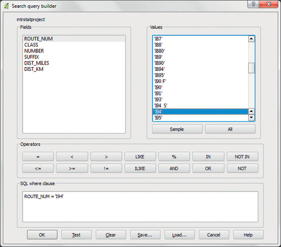
4. Select the intrstatproject layer in the Map Legend, open its attribute table, and bring up the query builder again. Build a query to select all lines with a route number equal to I94.
   

   (Source: QGIS)
5. The field that corresponds with route number is ROUTE_NUM.
6. Click All to show all available values.
7. Select = for the Operator, then from the Values table choose ‘I94’ (note that QGIS doesn’t necessarily sort all values in numerical order).
8. Click OK when the query is built. Zoom out so that you can see the length of I-94 (a major artery running east to west through the northern United States) on the screen.
9. Next, bring up the Buffer(s) dialog and create a 32186.9-meter (20-mile) buffer around the selected features of I-94. Set the Segments to approximate option to 20. Be sure to select the Dissolve buffer results option and choose the Use only selected features option. Call the output shapefile I94_20milebuffer.shp.
   

   (Source: QGIS)
10. After the buffer is created, add it to the Map Legend.
11. Next, bring up the Select by location dialog and find which features in the citiesproject layer intersect the features of the I94_20milebuffer layer by creating a new selection.
    

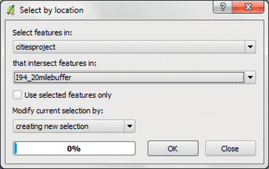    (Source: QGIS)
12. Select the citiesproject layer from the Map Legend, then open the attribute table for the cities and view the selected results.

    Question 6.3

    uuB3lcqt8yH4hcXRzLKDRfRGX+E4NOYfG5eKox2GnaLQIzSGKxkujvdK/+jpMC62
13. Unselect all of the selected cities and redo the analysis, this time with a 16093.4-meter (i.e., 10-mile) buffer. Be sure to use 20 Segments to approximate, and to dissolve the buffer results. Create a new output shapefile called I94_10milebuffer and find which cities intersect this new buffer as a new selection.

    185

    Question 6.4

    pdm2YU1z/Eo5JJ9xUNoR2n0Wx3TbCFb3MWHejHPGZbA0Yk5s7RauIyWcVL+IN3xH
14. Unselect all of the selected cities and redo the analysis one more time, this time with a 8046.72-meter (i.e., 5-mile) buffer. Be sure to use 20 Segments to approximate and to dissolve the buffer results. Create a new output shapefile called I94_5milebuffer and find which cities intersect this new buffer as a new selection.

    Question 6.5

    s3D+3Gwe8XvCEXkDF9wfgH+D4ZupcPCYr7lUuo8rbdO6nVj1hDDfjFaK3Y9+D99E
15. Unselect all of the currently selected features and turn off the buffers.

6.5 Selecting by Location with Polygons

1. For your next question, you’ll want to know how many cities are within states that have a high population. Unfortunately, the states layer only has total population values, and gives no information about numbers of cities or populated places. However, this type of question can be answered spatially using the query builder and select by location tools that you’ve been using so far in this lab.
2. In the Map Legend, select the statesproject layer, open its attribute table, and bring up the query builder dialog box.
3. Construct a query that will select all states with a year 2005 population (the Field is called POP2005) of greater than 2,000,000 persons.
   

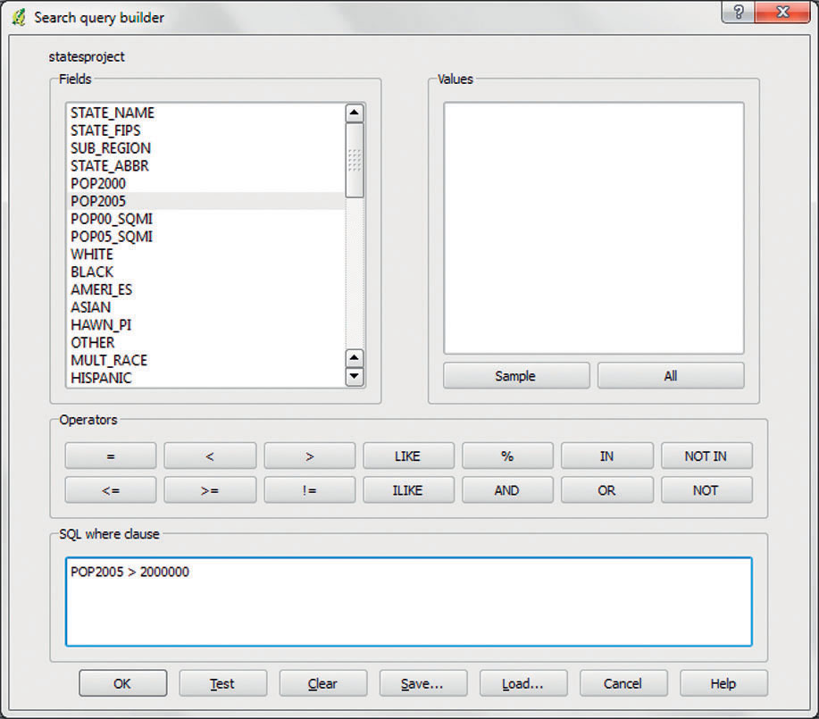   (Source: QGIS)
4. Click OK when the query is ready.

   Question 6.6

   MKwRz/bq3j/F8P3/LyyBXr6j/tdfwQYqhStHT1bbo06tpzy/sQRssbswgV6QC3fASyMsGTzCCgyDnUO/iS9WX8feNluIFVQ3wortQiKO9cPKlgaC
5. Next, bring up the Select by location tool to select cities that intersect one of these selected states (that have a population of more than 2,000,000 persons).
   

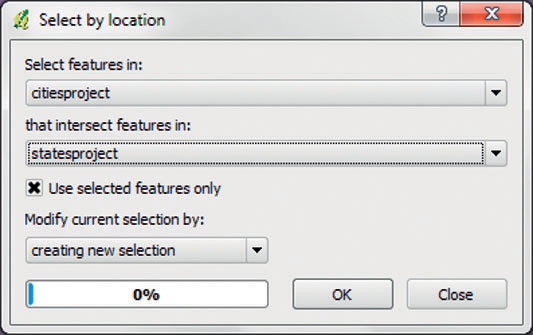   (Source: QGIS)
6. You’ll want to select features from the citiesproject layer that intersect features in the statesproject layer. Also be sure to use the selected features only (since you only want to locate which cities are within one of the high population states you just selected). Click OK when the settings are correct.
7. Answer Question 6.7 (this will involve examining the selected cities in the attribute table).

   Question 6.7

   Kf++5777ssuUdz19EHT4GbMz7Lg74C32o3Zzmj9p1P3VFiEAuieRxeSjkgL0fDknGGt6FwNC4ZC8KQWycMwKN2XqE/uu9qRdkOMLBcM7XTnXeThhD2jpjy1Xns5z4jLqLzqEx6tRfzTM5/z1LW+keOa5rZ42GmXSW0K3479ZseO9WVOkprC/Zg==
8. Unselect all of the currently selected features from both the citiesproject and the statesproject layers.

6.6 More Spatial Analysis

1. The next analysis that you’ll perform involves analysis of the features in relation to the Great Lakes, so zoom in on the Map View so that you can see all five Great Lakes. The first thing you’ll need to do is select the Great Lakes to work with.
2. Select the lakesproject shapefile in the Map Legend, open its attribute table and bring up the query builder. You’ll see that the two available fields that are available for query are the Name and Area of the lake records. You’ll want to build a query that looks for the name of each of the five Great Lakes as follows: NAME = ‘Lake Erie’ OR NAME = ‘Lake Huron’ OR NAME = ‘Lake Michigan’ OR NAME = ‘Lake Ontario’ OR NAME = ‘Lake Superior’.

   187

   

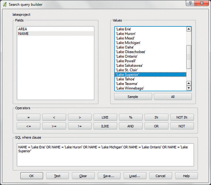   (Source: QGIS)
3. Answer Question 6.8, and then click OK. All five Great Lakes will now be selected.

   Question 6.8

   K2aA3FQ98BpYfknTL7uY6Zgzf2pPW+CgW7o4RDC9lZRZF1o7J/GwcEfy6uh2q6xnPeSDm+QfNKoqJCt2PPjBDzgzB9PD7MaX82+nAsWJs670MQVrVms3kISxit2ZwcKN4aiwI1DwYFJvt3I8v/V0c5HP/M3m7fzIRK36T3QIAbwG94aYGRu7M+JuYDKz//Bicys66iiSJQdL4LH/J0pOGAyK4Ebinl3Ge5ro61E85g+Qetm7luF34mQOf9cA493FV3u8nA==
4. Next, bring up the Buffer(s) dialog, and find out how many rivers are within 5 miles (8046.72 meters) of the Great Lakes by creating a buffer called GL_5milebuffer and use select by location to find which features from the riversproject layer intersect it. Be sure to use 20 Segments to approximate and to dissolve the buffer results. Note that even if part of the river is within the 5-mile buffer, the entire river will be selected.

   Question 6.9

   B0J9O/8/gS92JXTRXwiup8PlmpD8h/5odab9avqhTAIyRjHqIgcUtoWvOKNyHlL5VEn3ypgz/mPLun1JQCAZUGl+vcdKFSrlZsMDKBZ7u5ZpkB8PYpzBhB4E1MIuePbDiVmTzvqxOHumU4LHmeBO2FmWI6M=
5. Lastly, use the GL_5milebuffer layer to find out how many cities are within 5 miles of the Great Lakes.

   Question 6.10

   l5XtE6Rk6AhG1Dwb1QmfSD2F04bT4jhLdOa+auxiy6iimSfQ3MQxzPUVlMXAy6qPYJfKqaxwwuvCutZd
6. Exit QGIS by selecting Exit from the File pull-down menu. There’s no need to save any data in this lab.

Closing Time

Now that you have the basics of working with GIS data down, and know how to perform some initial spatial analysis, the Geospatial Lab Application in Chapter 7 will describe how to take geospatial data and create a print-quality map, using QGIS or ArcGIS.