15.2 Statistical estimation using the sample proportion
Statistical inference uses sample data to draw conclusions about the entire population. Because good samples are chosen with random sampling, statistics such as computed from these samples are random variables. We can describe the behavior of a sample statistic by a probability model that answers the question “What would happen if we took random samples of the same size many times?” Here is an example that will lead us toward the probability ideas most important for statistical inference.
EXAMPLE 15.2: More Ohio Uninsured Drivers on the Road!

The proportion of uninsured drivers varies widely between states as do the enforcement policies. Maine and Massachusetts have the lowest rates in the nation, and both require drivers to show proof of insurance when they register a vehicle. Ohio is a passive enforcement state: although it requires drivers to indicate that they have insurance when they register a vehicle, no proof of insurance is required.3
The proportion p of Ohio drivers without insurance is a parameter describing the population of Ohio drivers. To estimate p, we take a simple random sample of 150 Ohio drivers and find that 27 do not have insurance. The sample proportion of these subjects without insurance is  = 27/150 = 0.18. It seems reasonable to use the sample result
= 0.18 to estimate the unknown p. An SRS should fairly represent the population, so the proportion
of the sample should be somewhere near the proportion p of the population. Of course, we don’t expect
to be exactly equal to p. We realize that if we choose another SRS, the sample will probably produce a different
.
= 27/150 = 0.18. It seems reasonable to use the sample result
= 0.18 to estimate the unknown p. An SRS should fairly represent the population, so the proportion
of the sample should be somewhere near the proportion p of the population. Of course, we don’t expect
to be exactly equal to p. We realize that if we choose another SRS, the sample will probably produce a different
.
336
If
is rarely exactly right and varies from sample to sample, why is it nonetheless a reasonable estimate of the population proportion p? Here is one answer: if we continue to take larger and larger samples, the statistic
is guaranteed to get closer and closer to the parameter p. We have the comfort of knowing that if we can afford to continue sampling more subjects, eventually we will estimate the proportion of uninsured Ohio drivers very accurately. This is a special case of a more general mathematical result called the law of large numbers that we will encounter in Chapter 19.
Law of Large Numbers for Proportions
Draw observations at random from any population with population proportion p. As the number of observations drawn increases, the sample proportion
gets closer and closer to the population proportion p.
You should recognize the similarity between the law of large numbers for proportions and the idea of probability (page 260). The idea of probability states that in the long run, the proportion of outcomes taking any value gets close to the probability of that value. Suppose the value of the outcome corresponds to obtaining a success when sampling a single individual from the population. Then the probability of the value of the outcome is p, the proportion of successes in the population. The fact that
gets closer and closer to the population proportion p is just the idea of probability rephrased in our new terminology. Because of the importance of this concept, here is an example similar to Example 11.2 (page 260), but in the context of inference.
EXAMPLE 15.3: The Law of Large Numbers for Proportions in Action
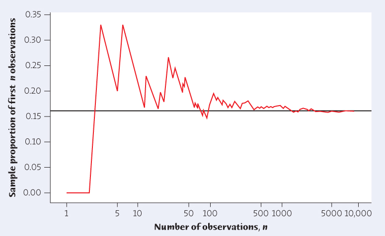
Extensive studies conducted throughout the year show that the proportion of uninsured drivers in Ohio is very close to 16%.4 Because of this, we will take p = 0.16 as the value of the population proportion, or the true value of the parameter. Figure 15.1 shows how the sample sample proportion
of an SRS drawn from the population of drivers changes as we add more subjects to our sample.
 always approaches the population proportion p.
337
The first subject in the sample had insurance, so the sample proportion after sampling one subject is zero, and the line in Figure 15.1 starts there. The second subject also had insurance, and the sample proportion after sampling two subjects remains at zero as in Figure 15.1. The third subject did not have insurance, so after sampling three subjects the sample proportion increases to
the third point on the graph. At first, the graph shows that the sample proportion changes considerably as we take more observations. Eventually, however, the sample proportion gets close to the population proportion p = 0.16 and settles down to that value.
If we started over, again choosing people at random from the population, we would get a different path from left to right in Figure 15.1. The law of large numbers says that whatever path we get will always settle down to 0.16 as we draw more and more people.
We know that if we continue to sample subjects, eventually we will estimate the population proportion very accurately. In practice, we take a sample of a fixed size. The key idea that will allow us to calculate the accuracy of an estimate for a fixed sample size is presented in the next section.
Apply Your Knowledge
Question 15.4
Prayer Among the Millennials. The Millennial generation (so called because they were born after 1980 and began to come of age around the year 2000) are less religiously active than older Americans. One of the questions in the General Social Survey in 2012 was “How often does the respondent pray?” Among the 377 respondents in the survey between 18 and 30 years of age, 225 prayed at least once a week.5
- (a) Describe the population and explain in words what the parameter p is.
- (b) Give the numerical value of the statistic
that estimates p.
Question 15.5
 The Law of Large Numbers for Proportions Made Visible. You are going to simulate sampling from a population with proportion of successes p = 0.16 as in Example 15.3. The law of large numbers says that the proportion
from a sample gets closer and closer to p = 0.16 as the sample increases in size.
The Law of Large Numbers for Proportions Made Visible. You are going to simulate sampling from a population with proportion of successes p = 0.16 as in Example 15.3. The law of large numbers says that the proportion
from a sample gets closer and closer to p = 0.16 as the sample increases in size.
- (a) The Probability applet can simulate sampling from a population with any proportion of successes. Set the probability of heads to 0.16 and the number of tosses to 50 using the sliders. Then check “Show true probability” to show this value on the graph. Now click “Toss.” You see that the graph displays at each point the proportion of successes up to the last one. This is exactly like Figure 15.1. What is the value of after 50 tosses? This will be to the right of “heads =” in the window.
- (b) Click “Toss” again to generate 50 more observations—don’t click “Reset.” Repeat this one more time so that there are now a total of 150 observations. What changes do you notice after clicking “Toss” each time in the graph? What portion of your final graph is similar to Figure 15.1? Is there any portion of the graph that is different? Sketch (or print out) the final graph.
338