Question 1 of 14
Step 1
Consider the following graph for a firm that can choose either to behave as a competitive firm or act as a monopolist. The marginal cost (MC) curve, the marginal revenue (MR) curve, and the demand (D) curve corresponding to each level of output (Q) and price (P) are shown in the graph below.
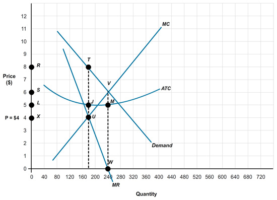
Under monopoly, the firm would follow the pricing rule , which is found at point .
Step 2

The firm would produce units at a price of .
Step 3

Profit would be depicted by the bounded by .
Step 4

Deadweight loss would be depicted by the bounded by .
Step 5

How much is the firm’s revenue? $
Step 6

How much are the firm’s costs? $
Step 7

How much are the firm’s profits? $
Step 8

Under perfect competition, the firm would follow the pricing rule , which is found at point .
Step 9

The firm would produce units at a price of .
Step 10

In the long run, profit would be .
Step 11

Deadweight loss would be .
Step 12

How much is the firm’s revenue? $
Step 13

How much are the firm’s short-run costs? $
Step 14

How much are the firm’s short-run profits? $