TABLE OF CONTENTS

Question 1 of 8

Solved Problems
true
true
You must read each slide, and complete any questions on the slide, in sequence.

Consider the following aggregate supply-aggregate demand graph. The aggregate demand (AD) curve, short-run aggregate supply (SRAS) curve, and long-run aggregate supply (LRAS) curve are given in this graph.
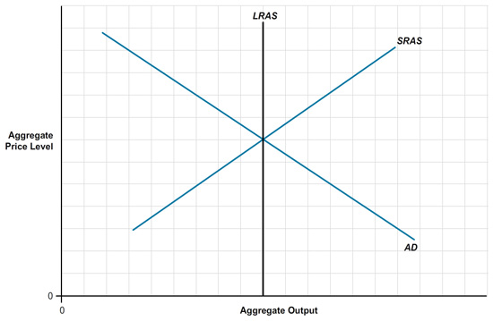
The horizontal axis is labeled Aggregate Output, and the vertical axis is labeled Aggregate Price Level. The graph shows the short-run aggregate supply curve, an upward sloping line labeled SRAS. The aggregate demand curve, labeled AD, is a downward sloping line that intersects the SRAS curve approximately in the center.  The long-run aggregate supply curve, labeled LRAS, is a vertical line that runs through the intersection of the SRAS and AD curves.

Factors that shift the aggregate demand curve left include .

Decreased consumer confidence reduces the consumption component of aggregate demand. The other choices either affect supply or increase aggregate demand.
3

The horizontal axis is labeled Aggregate Output, and the vertical axis is labeled Aggregate Price Level. The graph shows the short-run aggregate supply curve, an upward sloping line labeled SRAS. The aggregate demand curve, labeled AD, is a downward sloping line that intersects the SRAS curve approximately in the center.  The long-run aggregate supply curve, labeled LRAS, is a vertical line that runs through the intersection of the SRAS and AD curves.

After this shift, aggregate output , and the inflation rate .

If aggregate demand shifts left, aggregate output is lower (further left) and aggregate price level is lower as well.
3

The horizontal axis is labeled Aggregate Output, and the vertical axis is labeled Aggregate Price Level. The graph shows the short-run aggregate supply curve, an upward sloping line labeled SRAS. The aggregate demand curve, labeled AD, is a downward sloping line that intersects the SRAS curve approximately in the center.  The long-run aggregate supply curve, labeled LRAS, is a vertical line that runs through the intersection of the SRAS and AD curves.

Factors that shift the aggregate supply curve left include .

High oil prices raise business costs, forcing firms to either cut back or raise prices. This is represented by a leftward shift in aggregate supply. The other choices either affect demand or increase aggregate supply.
3

The horizontal axis is labeled Aggregate Output, and the vertical axis is labeled Aggregate Price Level. The graph shows the short-run aggregate supply curve, an upward sloping line labeled SRAS. The aggregate demand curve, labeled AD, is a downward sloping line that intersects the SRAS curve approximately in the center.  The long-run aggregate supply curve, labeled LRAS, is a vertical line that runs through the intersection of the SRAS and AD curves.

After this shift, aggregate output , and the aggregate price level .

If aggregate supply shifts left, aggregate output is lower (further left) and aggregate price level is higher.
3

The horizontal axis is labeled Aggregate Output, and the vertical axis is labeled Aggregate Price Level. The graph shows the short-run aggregate supply curve, an upward sloping line labeled SRAS. The aggregate demand curve, labeled AD, is a downward sloping line that intersects the SRAS curve approximately in the center.  The long-run aggregate supply curve, labeled LRAS, is a vertical line that runs through the intersection of the SRAS and AD curves.

Factors that shift the aggregate demand curve right include .

Increased government spending increases the ā€œGā€ component of aggregate demand. The other choices either affect supply or reduce aggregate demand.
3

The horizontal axis is labeled Aggregate Output, and the vertical axis is labeled Aggregate Price Level. The graph shows the short-run aggregate supply curve, an upward sloping line labeled SRAS. The aggregate demand curve, labeled AD, is a downward sloping line that intersects the SRAS curve approximately in the center.  The long-run aggregate supply curve, labeled LRAS, is a vertical line that runs through the intersection of the SRAS and AD curves.

After this shift, aggregate output , and the aggregate price level .

If aggregate demand shifts right, aggregate output is higher (further right) and aggregate price level is higher as well.
3

The horizontal axis is labeled Aggregate Output, and the vertical axis is labeled Aggregate Price Level. The graph shows the short-run aggregate supply curve, an upward sloping line labeled SRAS. The aggregate demand curve, labeled AD, is a downward sloping line that intersects the SRAS curve approximately in the center.  The long-run aggregate supply curve, labeled LRAS, is a vertical line that runs through the intersection of the SRAS and AD curves.

Factors that shift the aggregate supply curve right include .

Technological improvements allow firms to produce more output at a given price level. This results in aggregate supply moving right. The other choices either affect demand or reduce aggregate supply.
3

The horizontal axis is labeled Aggregate Output, and the vertical axis is labeled Aggregate Price Level. The graph shows the short-run aggregate supply curve, an upward sloping line labeled SRAS. The aggregate demand curve, labeled AD, is a downward sloping line that intersects the SRAS curve approximately in the center.  The long-run aggregate supply curve, labeled LRAS, is a vertical line that runs through the intersection of the SRAS and AD curves.

After this shift, aggregate output , and the aggregate price level .

If aggregate supply shifts right, aggregate output is higher (further right) but aggregate price level is lower. This can be explained as technology helping to produce more and cheaper goods.
3