Chapter 5. The Integral
Introduction
1
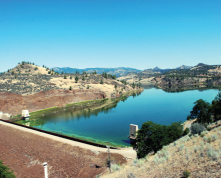
Managing the Klamath River
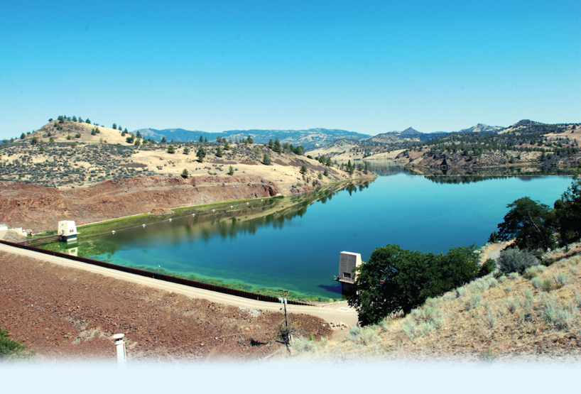
The Klamath River starts in the eastern lava plateaus of Oregon, passes through a farming region of that state, and then crosses northern California. Because it is the largest river in the region, and runs through a variety of terrain and has different land uses, it is important in a number of ways. Historically, the Klamath supported large salmon runs. It is used to irrigate agricultural lands, and to generate electric power for the region. Downstream, it runs through federal wild lands, and is used for fishing, rafting, and kayaking.
If a river is to be well-managed for such a variety of uses, its flow must be understood. For that reason, the U.S. Geological Survey (USGS) maintains a number of gauges along the Klamath. These typically measure the depth of the river, which can then be expressed as a rate of flow in cubic feet per second (ft3/s). In order to understand the river flow fully, one must be able to find the total amount of water that flows down the river over any period of time.
NOTE
The Chapter Project on page 62 examines ways to obtain the total flow over any period of time from data that provide flow rates.
We began our study of calculus by asking two questions from geometry. The first, the tangent problem, “What is the slope of the tangent line to the graph of of a function?” led to the derivative of a function.
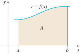
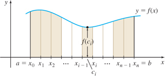
The second question was the area problem: Given a function f, defined and nonnegative on a closed interval [a,b], what is the area enclosed by the graph of f, the x-axis, and the vertical lines x=a and x=b? Figure 5.1 illustrates this area.
The first two sections of Chapter 5 show how the concept of the integral evolves from the area problem. At first glance, the area problem and the tangent problem look quite dissimilar. However, much of calculus is built on a surprising relationship between the two problems and their associated concepts. This relationship is the basis for the Fundamental Theorem of Calculus, discussed in Section 5.3.
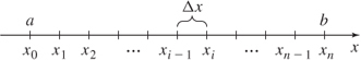
THIS PARA. IS A TEST ADDED BY JV: We divide, or partition, the interval [a,b] into n nonoverlapping subintervals: [x0,x1],[x1,x2],…,[xi−1,xi],…,[xn−1,xn] each of the same length. See Figure 5.7. Since there are n subintervals and the length of the interval [a,b] is b−a, the common length Δx of each subinterval is \boxed{\bbox[#FAF8ED,5pt]{\Delta x=\dfrac{b-a}{n}}}
5.1 Area
2
OBJECTIVES
When you finish this section, you should be able to:
- Approximate the area under the graph of a function (p. 2)
- Find the area under the graph of a function (p. 6)
In this section, we present a method for finding the area enclosed by the graph of a function y\,=\,f(x) that is nonnegative on a closed interval [a,b], the x-axis, and the lines x\,=\,a and x\,=\,b. The presentation uses summation notation (\sum ), which is reviewed in Appendix A.5.
5.1.1 Approximate the Area Under the Graph of a Function
The area A of a rectangle with base w and height l is given by the geometry formula \boxed{A\,=\,lw}
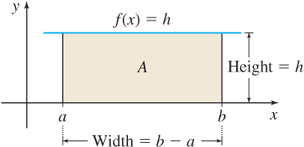
See Figure 5.2. The graph of a constant function f(x)\,=\,h, for some positive constant h, is a horizontal line that lies above the x-axis. The area enclosed by this line, the x-axis, and the lines x\,=\,a and x\,=\,b is the rectangle whose area A is the product of the base (b\,-\,a) and the height h. \boxed{A\,=\,(b\,-\,a)h} TEST
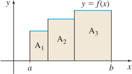
If the graph of y\,=\,f(x) consists of three horizontal lines, each of positive height as shown in Figure 5.3, the area A enclosed by the graph of f, the x-axis, and the lines x\,=\,a and x\,=\,b is the sum of the rectangular areas A_{1}, A_{2}, and A_{3}.
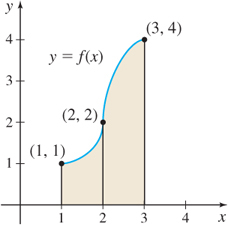
EXAMPLE 1 Approximating the Area Under the Graph of a Function
Approximate the area A enclosed by the graph of f(x) =\dfrac{1}{2}x+3, the x-axis, and the lines x=2 and x=4.
SolutionFigure 5.4 illustrates the area A to be approximated.
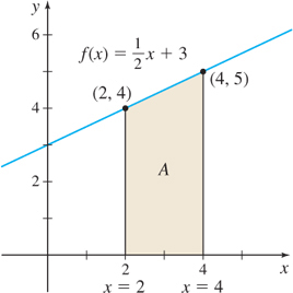
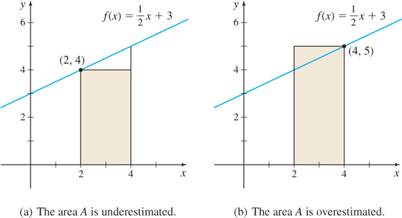
We begin by drawing a rectangle of base 4-2=2 and height f(2)=4. The area of the rectangle, 2\cdot 4=8, approximates the area A, but it underestimates A, as seen in Figure 5.5(a).
Alternatively, A can be approximated by a rectangle of base 4-2=2 and height f (4) =5. See Figure 5.5(b). This approximation of the area equals 2\cdot 5=10, but it overestimates A. We conclude that 8 \lt A \lt 10
3
The approximation of the area A can be improved by dividing the closed interval [2, 4] into two subintervals, [2, 3] and [3, 4]. Now we draw two rectangles: one rectangle with base 3-2=1 and height f(2) =\dfrac{1}{2}\cdot 2+3=4; the other rectangle with base 4-3=1 and height f (3) =\dfrac{1}{2}\cdot 3+3=\dfrac{9}{2}. As Figure 5.6(a) illustrates, the sum of the areas of the two rectangles 1\cdot 4+1\cdot \dfrac{9}{2}=\dfrac{17}{2}=8.5 underestimates the area.
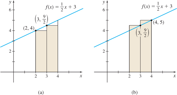
Now we repeat this process by drawing two rectangles, one of base 1 and height f(3) =\dfrac{9}{2}; the other of base 1 and height f(4) =\dfrac{1}{2}\cdot 4+3=5. As Figure 5.6(b) illustrates, the sum of the areas of these two rectangles, 1\cdot \dfrac{9}{2}+1\cdot 5=\dfrac{19}{2}=9.5
overestimates the area. We conclude that 8.5 \lt A \lt 9.5
obtaining a better approximation to the area.
NOTE
The actual area in Figure 5.4 is 9 sq units, obtained by using the formula for the area A of a trapezoid with base b and parallel heights h_{1} and h_{2}: A = \dfrac{1}{2}b ( h_{1} +h_{2}) =\dfrac{1}{2}(2) (4+5) = 9.
Observe that as the number of subintervals of the interval increases, the approximation of the area A improves. For n=1, the error in approximating A is 1 square unit, but for n=2, the error is only 0.5 square unit.
NOW WORK
Problem 5
In general, the procedure for approximating the area A is based on the idea of summing the areas of rectangles. We shall refer to the area A enclosed by the graph of a function y=f(x)\geq 0, the x-axis, and the lines x = a and x = b as the area under the graph of \boldsymbol{f} from \boldsymbol{a} to \boldsymbol{b}.
We make two assumptions about the function f:
- f is continuous on the closed interval [a,b].
- f is nonnegative on the closed interval [a,b].
We divide, or partition, the interval [a,b] into n nonoverlapping subintervals: \lbrack x_{0}, x_{1}], [x_{1}, x_{2}],\ldots , [x_{i-1},x_{i}],\ldots , [x_{n-1}, x_{n}] each of the same length. See Figure 5.7. Since there are n subintervals and the length of the interval [a,b] is b-a, the common length \Delta x of each subinterval is \boxed{\bbox[#FAF8ED,5pt]{\Delta x=\dfrac{b-a}{n}}}
4
NEED TO REVIEW?
The Extreme Value Theorem is discussed in Section 4.2, pp. xx-xx.
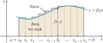
Since f is continuous on the closed interval [a,b], it is continuous on every subinterval [x_{i-1}, x_{i}] of [a,b]. By the Extreme Value Theorem, there is a number in each subinterval where f attains its absolute minimum. Label these numbers c_{1}, c_{2}, c_{3}, \ldots , c_{n}, so that f(c_{i}) is the absolute minimum value of f in the subinterval [x_{i-1}, x_{i}]. Now construct n rectangles, each having the \Delta x as its base and f(c_{i}) as its height, as illustrated in Figure 5.8. This produces n narrow rectangles of uniform width \Delta x=\dfrac{b-a}{n} and heights f(c_{1}), f(c_{2}), \ldots, f(c_{n}), respectively. The areas of the n rectangles are \begin{eqnarray*} \text{Area of the first rectangle} & = & f(c_{1})\Delta x \\ \text{Area of the second rectangle} & = & f(c_{2})\Delta x \\ & \vdots & \\ \text{Area of the }{n}\text{th} \text{ (and last) rectangle} & = & f(c_{n})\Delta x \end{eqnarray*}
The sum s_{n} of the areas of the n rectangles approximates the area A. That is, A\approx s_{n}=f(c_{\mathbf{1}})\Delta x+f(c_{\mathbf{2}})\Delta x+~\cdots~+f(c_{i})\Delta x+~\cdots ~+f(c_{n})\Delta x=\sum\limits_{i= 1}^{n}f(c_{i})\Delta x Since the rectangles used to approximate the area A lie under the graph of f, the sum s_{n}, called a lower sum, underestimates A. That is, s_{n}\leq A.
NEED TO REVIEW?
Summation notation is discussed in Appendix A.5, pp. A-38-A-43.
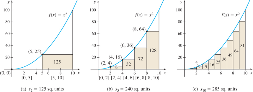
EXAMPLE 2 Approximating Area Using Lower Sums
Approximate the area A under the graph of f(x) = x^{2} from 0 to 10 by using lower sums s_{n} (rectangles that lie under the graph) for:
- n = 2 subintervals
- n = 5 subintervals
- n = 10 subintervals
Solution(a) For n=2, we partition the closed interval [0,10] into two subintervals [0,5] and [5,10], each of length \Delta x=\dfrac{10-0}{2}=5. See Figure 5.9(a). To compute s_{2}, we need to know where f attains its minimum value in each subinterval. Since f is an increasing function, the absolute minimum is attained at the left endpoint of each subinterval. So, for n=2, the minimum of f on [0,5] occurs at 0 and the minimum of f on [5,10] occurs at 5. The lower sum s_{2} is
5
s_{2}=\sum\limits_{i=1}^{2}~f(c_{i})\Delta x=\Delta x\sum\limits_{i=1}^{2}f(c_{i}) \underset{\underset{\underset{\color{#0066A7}{f\left(c_{1}\right) =f\left( 0\right) ;f\left( c_{2}\right) =f\left(5\right)}}{\color{#0066A7}{\Delta x=5}}}{\color{#0066A7}{\uparrow}}}{=}5\,\left[ ~f(0)+f(5)\right] \underset{\underset{\underset{\color{#0066A7}{f(5)=25}}{\color{#0066A7}{f(0)=0}}}{\color{#0066A7}{\uparrow}}}{=}5(0+25)=125
(b) For n=5, partition the interval [0,10] into five subintervals [0,2], [2,4], [4,6], [6,8], [8,10], each of length \Delta x = \dfrac{10-0}{5}=2. See Figure 5.9(b). The lower sum s_{5} is \begin{eqnarray*} s_{5} &=&\sum\limits_{i=1}^{5} f(c_{i})\Delta x=\Delta x\sum\limits_{i=1}^{5}f(c_{i})=2 [ f(0)+f(2)+f(4) +f(6)+f(8)] \\ &=&2( 0+4+16+36+64 ) =240 \end{eqnarray*}
(c) For n=10, partition [0,10] into 10 subintervals, each of length \Delta x=\dfrac{10-0}{10}=1. See Figure 5.9(c). The lower sum s_{10} is \begin{eqnarray*} s_{10} &=&\sum\limits_{i=1}^{10} f(c_{i})\Delta x=\Delta x\sum\limits_{i=1}^{10}f(c_{i})=1[ f(0)+f(1)+f(2)+\cdots +f(9) ] \\ &=&0+1+4+9+16+25+36+49+64+81=285 \end{eqnarray*}
NOW WORK
Problem 13(a).
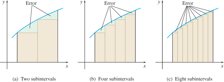
In general, as Figure 5.10(a) illustrates, the error due to using lower sums s_{n} (rectangles that lie below the graph of f) occurs because a portion of the area lies outside the rectangles. To improve the approximation of the area, we increased the number of subintervals. For example, in Figure 5.10(b), there are four subintervals and the error is reduced; in Figure 5.10(c), there are eight subintervals and the error is further reduced. So, by taking a finer and finer partition of the interval [a,b], that is, by increasing n, the number of subintervals, without bound, we can make the sum of the areas of the rectangles as close as we please to the actual area. (A proof of this statement is usually found in books on advanced calculus.)
In Section 5.3, we see that, for functions that are continuous on a closed interval, \lim\limits_{n\rightarrow \infty }s_{n} always exists. With this discussion in mind, we now define the area under the graph of a function f from a to b.
6
DEFINITION Area {A} Under the Graph of a Function from {a} to {b}
Suppose a function f is nonnegative and continuous on a closed interval [a,b]. Partition [a,b] into n subintervals [x_{0}, x_{1}], [x_{1}, x_{2}], \ldots, [x_{i-1}, x_{i}], \ldots, [x_{n-1}, x_{n}], each of length \Delta x=\dfrac{b-a}{n}
In each subinterval [ x_{i-1},x_{i}], let f (c_{i}) equal the absolute minimum value of f on this subinterval. Form the lower sums s_{n}=\sum\limits_{i= 1}^{n}f(c_{i})\Delta x=f(c_{\mathbf{1}})\Delta x+ \cdots +f(c_{n})\Delta x
The area \boldsymbol{A} under the graph of \boldsymbol{f} from \boldsymbol{a} to \boldsymbol{b} is the number \boxed{\bbox[5pt] {A=\lim\limits_{n\rightarrow \infty }s_{n} }}
The area A is defined using lower sums s_{n} (rectangles that lie below the graph of f). By a parallel argument, we can choose values C_{1}, C_{2}, \ldots , C_{n} so that the height f(C_{i}) of the ith rectangle is the absolute maximum value of f on the ith subinterval, as shown in Figure 5.11. The corresponding upper sums \boldsymbol{{S}_{n}} (rectangles that lie above the graph of f) overestimate the area A. So, S_{n}\geq A. It can be shown that as n increases without bound, the limit of the upper sums S_{n} equals the limit of the lower sums s_{n}. That is, \boxed{\bbox[#FAF8ED,5pt]{\lim\limits_{n\rightarrow \infty}s_{n}=\lim\limits_{n\rightarrow \infty }S_{n}=A }}
5.1.2 Find the Area Under the Graph of a Function
In the next example, instead of using a specific number of rectangles to approximate area, we partition the interval [a,b] into n subintervals, obtaining n rectangles. By letting n\rightarrow \infty, we find the actual area under the graph of f from a to b.
EXAMPLE 3 Finding Area Using Upper Sums
Find the area A under the graph of f(x) = 3x from 0 to 10 using upper sums S_{n} (rectangles that lie above the graph of f). Then A = \lim\limits_{n\rightarrow \infty }S_{n}.
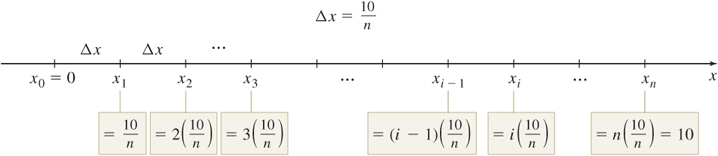
SolutionFigure 5.12 illustrates the area A. We partition the closed interval [0,10] into n subintervals {[{x_{0},x_{1}}]},\quad {[{x_{1},x_{2}}]}, \ldots, [x_{i-1},x_{i}] , \ldots ,\quad {{[{x_{n-1},x_{n}}]}}
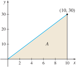
where 0=x_{0}\lt x_{1}\lt x_{2}\lt\cdots \lt x_{i}\lt\cdots \lt x_{n-1}\lt x_{n}=10
and each subinterval is of length \Delta x = {\dfrac{{10 - 0}}{{n}}} = {\dfrac{{10}}{{n}}}
The coordinates of the endpoints of each subinterval, written in terms of n, are \begin{eqnarray*} x_0 &=& 0,x_1 = \frac{{10}} {n},x_2 = 2\left( {\frac{{10}} {n}} \right), \ldots ,x_{i - 1} = (i - 1)\left( {\frac{{10}} {n}} \right), \\ x_i & =& i\left( {\frac{{10}} {n}} \right), \ldots ,x_n = n\left( {\frac{{10}} {n}} \right) = 10 \\ \end{eqnarray*}
as illustrated in Figure 5.13.
7
To find A using upper sums S_{n} (rectangles that lie above the graph of f), we need the absolute maximum value of f in each subinterval. Since f(x)=3x is an increasing function, the absolute maximum occurs at the right endpoint x_{i}= i\!\left(\dfrac{10}{n}\right) of each subinterval. So, \begin{eqnarray*} &S_{n}=\sum\limits_{i=1}^{n} f (C_i)&\Delta x = \sum \limits_{i=1}^{n}3x_{i}\cdot&\dfrac{10}{n} = {\sum\limits_{i=1}^{n}}\left( 3\cdot \dfrac{10i}{n}\right) \left(\dfrac{10}{n}\right) = \sum\limits_{i=1}^{n}\dfrac{300}{n^2}i \nonumber\\ &&\underset{\hbox{\(\color{#0066A7}{\Delta x = \dfrac{10}{n}}\)}}{\color{#0066A7}{\uparrow}} &\underset{\hbox{\(\color{#0066A7}{ {x}_{i} = \dfrac{10i}{n}}\)}}{\color{#0066A7}{\uparrow}} \end{eqnarray*}
RECALL
\sum\limits_{i=1}^{n}i=\dfrac{n(n+1)}{2}
Using summation properties, we get S_{n}= \sum\limits_{i=1}^{n} \dfrac{300}{n^2} i =\dfrac{300}{n^2} \sum\limits_{i=1}^{n} i = \dfrac{300}{n^2}\ \dfrac{n(n+1)}{2} = 150\left(\dfrac{n+1}{n}\right) =150\left(1+\dfrac{1}{n}\right)
Then A=\lim\limits_{n\rightarrow \infty }S_{n}=\lim\limits_{n\rightarrow \infty } \left[150 \left( 1+\dfrac{1}{n} \right) \right] =150\lim\limits_{n\rightarrow \infty }\left(1+\dfrac{1}{n}\right) =150
NEED TO REVIEW?
Summation properties are discussed in Appendix A.5, pp. A-38–A-43.
The area A under the graph of f(x)=3x from 0 to 10 is 150 square units.
NOTE
The area found in Example 3 is that of a triangle. So, we can verify that A=150 by using the formula for the area A of a triangle with base b and height h: A=\dfrac{1}{2}bh = \dfrac{1}{2} (10)(30) = 150 .
EXAMPLE 4 Finding Area Using Lower Sums
Find the area A under the graph of f(x) = 16 - x^{2} from 0 to 4 by using lower sums s_{n} (rectangles that lie below the graph of f). Then A=\lim\limits_{n\rightarrow \infty}{}s_{n}.
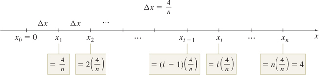
SolutionFigure 5.14 shows the area under the graph of f and a typical rectangle that lies below the graph. We partition the closed interval [0,4] into n subintervals {[{x_{0},x_{1}}]},\quad {[{x_{1},x_{2}}]}, \ldots , [x_{i-1},x_{i}], \ldots , {[{x_{n-1},x_{n}}]}
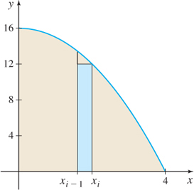
where 0=x_{0}\lt x_{1}\lt \cdots \lt x_{i}\lt \cdots \lt x_{n-1} \lt x_{n}=4
and each interval is of length \Delta x = \dfrac{{4-0}}{n} = \dfrac{4}{n}
As Figure 5.15 illustrates, the endpoints of each subinterval, written in terms of n, are \begin{array}{l} {x_0 = 0,x_1 = 1\left( {\frac{4} {n}} \right),x_2 = 2\left( {\frac{4} {n}} \right), \cdots ,x_{i - 1} = (i - 1)\left( {\frac{4} {n}} \right),} \\ {x_i = i\left( {\frac{4} {n}} \right), \cdots ,x_n = n\left( {\frac{4} {n}} \right) = 4} \\ \end{array}
8
To find A using lower sums s_{n} (rectangles that lie below the graph of f), we must find the absolute minimum value of f on each subinterval. Since the function f is a decreasing function, the absolute minimum occurs at the right endpoint of each subinterval. So, s_{n}={\sum\limits_{i=1}^{n}} f (c_{i})\Delta x
Since c_{i}=i\!\left( \dfrac{4}{n}\right) =\dfrac{4i}{n} and \Delta x=\dfrac{4}{n}, we have \begin{array}{l} {s_n } & { = \sum\limits_{i = 1}^n {f(c_i )\Delta x = \sum\limits_{i = 1}^n {\left[ {16 - \left( {\frac{{4i}} {n}} \right)^2 } \right]} \underset{\color{#0066A7}{f(c_i ) = 16 - c_i^2 ;c_i = \frac{{4i}}{4}}}{\left( {\frac{4} {n}} \right)} }} \\ {} & { = \sum\limits_{i = 1}^n {\left[ {\frac{{64}} {n} - \frac{{64i^2 }} {{n^3 }}} \right]} } \\ {} & { = \frac{{64}} {n}\sum\limits_{i = 1}^n {1 - \frac{{64}} {{n^3 }}\sum\limits_{i = 1}^n {i^2 } } } \\ {} & { = \frac{{64}} {n}(n) - \frac{{64}} {{n^3 }}\left[ {\frac{{n(n + 1)(2n + 1)}} {6}} \right] = 64 - \frac{{32}} {{3n^2 }}[2n^2 + 3n + 1]} \\ {} & { = 64 - \frac{{64}} {3} - \frac{{32}} {n} - \frac{{32}} {{3n^2 }} = \frac{{128}} {3} - \frac{{32}} {n} - \frac{{32}} {{3n^2 }}} \\ \end{array}
RECALL
\sum\limits_{i=1}^{n} 1=n; \sum\limits_{i=1}^{n} {i}^{2} = \dfrac{{n}({n+1}) (2n+1)}{6}
Then A=\lim\limits_{n\rightarrow \infty }s_{n}={\lim\limits_{n\rightarrow \infty } }\left( {{\dfrac{{128}}{{3}}}}-{{\dfrac{{32}}{{n}}}-{\dfrac{{32}}{{3n^{2}}}}} \right) ={\dfrac{{128}}{{3}}}
The area A under the graph of f (x) =16-x^{2} from 0 to 4 is \dfrac{128}{3} square units.
NOW WORK
Problem 29
The previous two examples illustrate just how complex it can be to find areas using lower sums and/or upper sums. In the next section, we define an integral and show how it can be used to find area. Then in Section 5.3, we present the Fundamental Theorem of Calculus, which provides a relatively simple way to find area.
5.2 Assess Your Understanding
Concepts and Vocabulary
Question 5.1
Explain how rectangles can be used to approximate the area enclosed by the graph of a function y=f(x) \geq 0, the x-axis, and the lines x=a and x=b.
Question 5.2
True or False When a closed interval [a,b] is partitioned into n subintervals each of the same length, the length of each subinterval is \dfrac{a+b}{n}.
Question 5.3
If the closed interval [-2,4] is partitioned into 12 subintervals, each of the same length, then the length of each subinterval is _________.
Question 5.4
True or False If the area A under the graph of a function f that is continuous and nonnegative on a closed interval [a,b] is approximated using upper sums S_{n}, then S_{n}\geq A and A=\lim\limits_{n\rightarrow \infty }S_{n}.
9
Skill Building
Question 5.5
Approximate the area A enclosed by the graph of f(x) = \dfrac{1}{2}x+3, the x-axis, and the lines x=2 and x=4 by partitioning the closed interval [2, 4] into four subintervals: \left[ 2, \dfrac{5}{2}\right], \left[ \dfrac{5}{2},3 \right], \left[3, \dfrac{7}{2}\right], \left[ \dfrac{7}{2}, 4\right].
- Using the left endpoint of each subinterval, draw four small rectangles that lie below the graph of f and sum the areas of the four rectangles.
- Using the right endpoint of each subinterval, draw four small rectangles that lie above the graph of f and sum the areas of the four rectangles.
- Compare the answers from parts (a) and (b) to the exact area A=9 and to the estimates obtained in Example 1.
Question 5.6
Approximate the area A enclosed by the graph of f(x) =6-2x, the x-axis, and the lines x=1 and x=3 by partitioning the closed interval [ 1,3] into four subintervals: \left[1, \dfrac{3}{2}\right], \left[ \dfrac{3}{2},2\right], \left[ 2,\dfrac{ 5}{2}\right], \left[ \dfrac{5}{2},3\right].
- Using the right endpoint of each subinterval, draw four small rectangles that lie below the graph of f and sum the areas of the four rectangles.
- Using the left endpoint of each subinterval, draw four small rectangles that lie above the graph of f and sum the areas of the four rectangles.
- Compare the answers from parts (a) and (b) to the exact area A=4.
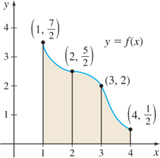
In Problems 7 and 8, refer to the illustrations. Approximate the shaded area under the graph of f from 1 to 3:
- By constructing rectangles using the left endpoint of each subinterval.
- By constructing rectangles using the right endpoint of each subinterval.
Question 5.7
Question 5.8
In Problems 9-12, partition each interval into n subintervals each of the same length.
Question 5.9
[1,4] with n = 3
Question 5.10
[0,9] with n = 9
Question 5.11
[{-}1,4] with n = 10
Question 5.12
[{-}4,4] with n = 16
In Problems 13 and 14, refer to the graphs. Approximate the shaded area:
- By using lower sums s_{n} (rectangles that lie below the graph of f).
- By using upper sums S_{n} (rectangles that lie above the graph of f).
Question 5.13
Question 5.14
5.3 The Definite Integral
11
OBJECTIVES
When you finish this section, you should be able to:
- Define a definite integral as the limit of Riemann sums (p. 11)
- Find a definite integral using the limit of Riemann sums (p. 14)
The area A under the graph of y = f(x) from a to b is obtained by finding \begin{equation} \boxed{\bbox[#FAF8ED,5pt]{{A=\lim\limits_{n\rightarrow \infty}s_{n}=\lim\limits_{n\rightarrow \infty }{\sum\limits_{i=1}^{n}} {f}(c_{i}) \Delta x=\lim\limits_{n\rightarrow \infty }S_{n}=\lim\limits_{n\rightarrow \infty }{\sum\limits_{i=1}^{n}} {f}(C_{i}) \Delta x }}} \end{equation}
THEOREM The Integral of the Sum of Two Functions
If two functions f and g are continuous on the closed interval [a,b], then \begin{equation*} \boxed{\bbox[5pt]{\int_{a}^{b}[ f(x)+g(x)] \,dx=\int_{a}^{b}f(x)\,dx+\int_{a}^{b}g(x)\,dx}}\tag{1} \end{equation*}
Chapter Review
58
THINGS TO KNOW
5.1 Area
Definitions:
- Partition of an interval [a,b] (p. xx)
- Area A under the graph of a function f from a to b (p.xx)
5.2 The Definite Integral
Definitions:
- Riemann sums (p. xx)
- The definite integral (p. xx)
- \int_{a}^{a}f(x)\,dx=0 (p. xx)
- \int_{a}^{b}f(x)\,dx=-\int_{b}^{a}f(x)\,dx (p. xx)
Theorem: If a function f is continuous on a closed interval [a,b], then the definite integral \int_{a}^{b}f(x)\,dx exists. (p. xx)
- \int^b_a h\ dx = h(b-a), h a constant
59
OBJECTIVES
| Section | You should be able to … | Examples | Review Exercises |
|---|---|---|---|
| 5.1 | 1 Approximate the area under the graph of a function (p.xx) | 1, 2 | 1, 2 |
| 2 Find the area under the graph of a function (p.xx) | 3–5 | 3, 4 | |
| 5.2 | 1 Define a definite integral as the limit of Riemann sums (p. xx) | 1–2 | 5(a), (b) |
| 2 Find a definite integral using the limit of Riemann sums (p. xx) | 3–5 | 5(c), 6 | |
| 5.3 | 1 Use Part 1 of the Fundamental Theorem of Calculus (p. xx) | 1–3 | 7-10, 59 |
| 2 Find a definite integral using Part 2 of the Fundamental Theorem of Calculus (p. xx) | 4, 5 | 5(d), 11–13, 17, 18, 63 | |
| 3 Interpret an integral using Part 2 of the Fundamental Theorem of Calculus (p. xx) | 6 | 21, 22 | |
| 5.4 | 1 Use properties of the definite integral (p. xx) | 1–6 | 15, 16, 23, 24, 27, 28, 60, 64 |
| 2 Work with the Mean Value Theorem for Integrals (p. xx) | 7 | 29, 30 | |
| 3 Find the average value of a function (p. xx) | 8 | 31–36 | |
| 5.5 | 1 Find indefinite integrals (p. xx) | 1 | 14 |
| 2 Use properties of indefinite integrals (p. xx) | 2, 3 | 19, 20, 37, 38 | |
| 3 Solve differential equations involving growth and decay (p. xx) | 4, 5 | 39, 40, 66, 67 | |
| 5.6 | 1 Find an indefinite integral using substitution (p. xx) | 1–5 | 42–45, 49, 50, 53, 54, 57, 58 |
| 2 Find a definite integral using substitution (p. xx) | 6, 7 | 46–48, 51, 52, 55, 56, 61, 62 | |
| 3 Integrate even and odd functions (p. xx) | 8, 9 | 25–28 | |
| 4 Solve differential equations: Newton's Law of Cooling (p. xx) | 10 | 65 |
CHAPTER 5 PROJECT Managing the Klamath River
There is a gauge on the Klamath River, just downstream from the dam at Keno, Oregon. The U.S. Geological Survey has posted flow rates for this gauge every month since 1930. The averages of these monthly measurements since 1930 are given in Table 2. Notice that the data in Table 2 measure the rate of change of the volume V in cubic feet of water each second over one year; that is, the table gives \dfrac{dV}{dt}=V^\prime (t) in \hbox{cubic feet per second}, where t is in months.
| Month | Flow Rate ({\bf ft}^{\bf 3}/{\bf s}) |
|---|---|
| January (1) | 1911.79 |
| February (2) | 2045.40 |
| March (3) | 2431.73 |
| April (4) | 2154.14 |
| May (5) | 1592.73 |
| June (6) | 945.17 |
| July (7) | 669.46 |
| August (8) | 851.97 |
| September (9) | 1107.30 |
| October (10) | 1325.12 |
| November (11) | 1551.70 |
| December (12) | 1766.33 |
Question 5.15
Find the factor that will convert the data in Table 2 from seconds to days. [Hint: 1 day =1\text {d} =24 \text{ hours } =24\text{h} (60\text{min}/\text{h}) = (24)(60)\text{min} (60\text{s}/\text{min}).]
If we assume February has 28.25 days, to account for a leap year, then 1 year =365.25 days. If V^\prime (t) is the rate of flow of water, in \hbox{cubic feet per day}, the total flow of water over 1 year is given by V=V(t) =\int_{0}^{365.25}V^\prime (t) dt.