CHAPTER 14 PROJECT The Mass of Stars

The mass of a star is distributed throughout its volume and can be described by its density \(\delta\)* measured in \(\text{kg}/\text{m}^{3}\). However, while solids often have constant density, the density of a star varies with respect to position within the star’s volume. A triple integral can then be used to find the mass \(M\) of the star provided its density function is known. We examine several possible density functions for stars. Because stars are almost spherical, we use spherical coordinates and position the sphere so that its center is at the origin.

• 1. Show that the mass \(M\) of a solid enclosed by a sphere of radius \(R \text{m}\) and constant density \(\delta\) is given by \(M=\dfrac{4}{3}\delta \pi R^{3}.\)

  While we can model the shape of a star as a sphere, its density \(\delta \) is not constant. Gravitational forces between the gaseous particles in the star cause the density to be greatest near the center of the star, to become less dense further from its center, and to eventually become zero at the edge of the star. There are various ways to model the density \(\delta\) of a star as a function of the radial distance \(\rho \) from the star’s center.

  Here, we examine three of these models and use each to determine the mass \(M\) of a star. For each these models, \(R\) is the radius of the star, \(\delta _{0}\) is a constant, and \(\rho\) is the radial distance from the center of the star.

  972

  The linear density model is given by \[ \delta ( \rho ) =\delta _{0}\left( 1-\dfrac{\rho }{R}\right) \]

• 2. Show that the linear density model satisfies the condition that the density at the edge of the star is \(0.\)

• 3. Show also that in the linear density model the constant \(\delta _{0}\) equals the density at the center of the star.

• 4. Find the mass \(M\) of a star that obeys the linear density model.

  The quadratic density model is given by \[ \delta ( \rho ) =\delta _{0}\left[ 1-\left( \dfrac{\rho }{R} \right) ^{2}\right] \]

• 5. Show that the quadratic density model satisfies the condition that the density at the edge of the star is \(0.\)

• 6. Show also that in the quadratic density model the constant \(\delta _{0}\) equals the density at the center of the star.

• 7. Find the mass \(M\) of a star that obeys the quadratic density model.

  A third model for the density involves an exponential decrease in mass density. In this exponential density model the density \(\delta =\delta (\rho)\) of a star is given by \[ \delta ( \rho ) =\delta _{0}[ e^{( 1-\rho /R) }-1] \]

• 8. Show that this exponential density model satisfies the condition that the density at the edge of the star is \(0\).

• 9. Show that the density at the center of a star modeled by the exponential model is \(\delta _{0}(e-1) \text{kg}/\text{m}^{3}.\)

• 10. Find the mass \(M\) of a star that obeys the exponential model.

• 11. Using each of the three models, integrate over a volume with radius \( \rho \) \(\lt R\) to find an expression for the mass of the star contained within a region of radius \(\rho\) about its center. Compare how the mass of a star differs in each of these models at a fixed radial distance \(\rho _{0}.\) This is a way to see how the mass within the interior of the star grows as the radial distance from the center increases.

  It should not be a surprise that the structure of a real star is vastly more complicated than the models above indicate.

  The mass of a star at any radial distance \(\rho \) is governed by the differential equation of mass conservation, \[ \dfrac{d}{d\rho }M(\rho) =4\pi \rho ^{2}\delta (\rho) \]

  The balance of gas pressure \(P\), which tends to blow the star apart, and gravity, which in the absence of pressure would make the star collapse, gives us the differential equation of hydrostatic equilibrium \[ \dfrac{dP}{d\rho }=-G\dfrac{M(\rho) \,\delta }{\rho ^{2}} \]

  To these equations we add an equation for the conservation of energy, and an equation that governs the energy transport from the center to the surface. These form a set of four basic coupled differential equations which, for a given stellar mass and composition of elements, can be integrated numerically to give the run of pressure, temperature, mass and energy distribution through the star. As Figure 66 indicates, there are other complicating factors.

  

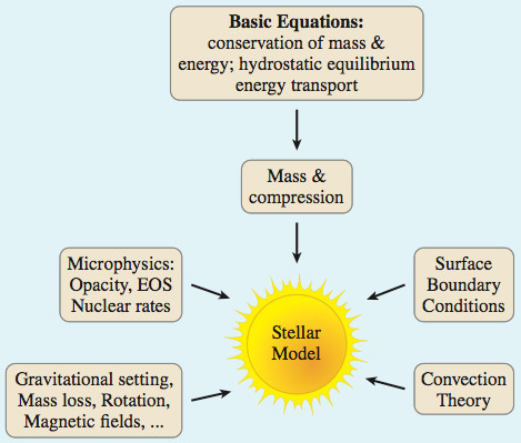  Figure 66

  Source: Brian Chaboyer, Dartmouth College

  Through literally hundreds of years of careful observation, increasingly sophisticated understanding of the relevant physics, and more and more powerful mathematical techniques, astronomers now have a fairly complete understanding of stellar structure and evolution. It continues as an active area of research, and is one of the beautiful triumphs of mathematics.