2.1 Rates of Change and the Derivative
145
OBJECTIVES
When you finish this section, you should be able to:
- Find instantaneous velocity (p. 145)
- Find an equation of the tangent line to the graph of a function (p. 147)
- Find the rate of change of a function (p. 149)
- Find the derivative of a function at a number (p. 150)
Everything in nature changes. Examples include climate change, change in the phases of the moon, and change in populations. To describe natural processes mathematically, the ideas of change and rate of change are often used. In this section, we use a limit to describe a rate of change and discover that seemingly unrelated interpretations of rates of change have a common basis we call a derivative.
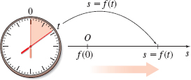
Average velocity provides a physical example of an average rate of change. For example, consider an object moving along a horizontal line with the positive direction to the right, or moving along a vertical line with the positive direction upward. Motion of this sort is referred to as rectilinear motion. The object’s location at time \(t=0\) is called its initial position. The initial position is usually marked as the origin O on the line. See Figure 1. We assume the distance \(s\) at time \(t\) of the object from the origin is given by a function \( s=f( t)\). Here, \(s\) is the signed, or directed, distance (using some measure of distance such as centimeters, meters, feet, etc.) of the object from O at break time \(t\) (in seconds or hours).
spanDEFINITIONspan Average Velocity
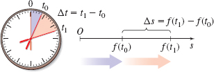
The (signed) distance \(s\) from the origin at time \(t\) of an object in rectilinear motion is given by the function \(s=f( t)\). If at time \(t_{0}\) the object is at \(s_{0}=f( t_{0})\) and at time \( t_{1}\) the object is at \(s_{1}=f( t_{1})\), then the change in time is \(\Delta t=t_{1}-t_{0}\) and the change in distance is \(Δ s=s_{1}-s_{0}=f( t_{1}) -f( t_{0})\). The average rate of change of distance with respect to time is \[\bbox[5px, border:1px solid black, #F9F7ED]{ \dfrac{\Delta s}{\Delta t}=\dfrac{f( t_{1}) -f( t_{0}) }{t_{1}-t_{0}}\qquad t_{1}\neq t_{0}} \]
and is called the average velocity of the object over the interval \([ t_{0},t_{1}]\).
See Figure 2.
Finding Average Velocity
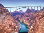
The Mike O’Callaghan-Pat Tillman Memorial Bridge spanning the Colorado River opened on October 16, 2010. Having a span of 1900 feet, it is the longest arch bridge in the Western Hemisphere, and its roadway is 890 feet above the Colorado River.
NOTE
Here, the motion occurs along a vertical line with the positive direction downward.
If a rock falls from the roadway, the function \(s=\) \(f(t) =16t^{2}\) gives the distance \(s\), in feet, that the rock falls after \(t\) seconds for \(0 ≤ t ≤ 7.458\). Here, \(7.458\) seconds is the approximate time it takes the rock to fall \(890\) feet into the river. The average velocity of the rock during its fall is \[ \dfrac{\Delta s}{\Delta t}=\dfrac{f( 7.458) -f(0) }{7.458-0}=\dfrac{890-0}{7.458}\approx 119.335\; \hbox{feet per second} \]
1 Find Instantaneous Velocity
The average velocity of the rock in Example 1 approximates the average velocity over the interval \([0,7.458].\) But the average velocity does not tell us about the velocity at any particular instant of time. That is, it gives no information about the rock’s instantaneous velocity.
146
NOTE
Speed and velocity are not the same thing. Speed measures how fast an object is moving and is defined as the absolute value of its velocity. Velocity measures both the speed and the direction of an object and may be a positive or a negative number or zero.
We can investigate the instantaneous velocity of the rock, say, at \(t=3\) seconds, by computing average velocities for short intervals of time beginning at \(t=3\). First we compute the average velocity for the interval beginning at \(t=3\) and ending at \(t=3.5\). The corresponding distances the rock has fallen are \[ f(3) =16\cdot 3^{2}=144\; \hbox{feet when}\; t=3\;\hbox{seconds} \]
and \[ f( 3.5) =16\cdot (3.5)^{2}=196\; \hbox{feet when}\; t=3.5\;\hbox{seconds} \]
Then \(\Delta t=3.5-3.0=0.5\), and during this 0.5-second interval,
Average velocity \(=\dfrac{\Delta s}{\Delta t}=\dfrac{f( 3.5) -f(3) }{3.5-3}=\dfrac{196-144}{0.5}=104\) feet per second
Table 1 shows average velocities of the rock for smaller intervals of time.
| Time interval | Start \({t}_{0}= 3\) | End \(t\) | \({\Delta t}\) | \(\dfrac{\Delta s}{\Delta t}=\dfrac{f(t) -f( t_{0})}{t-t_{0}}=\dfrac{16t^{2}-144}{t-3}\) |
|---|---|---|---|---|
| [3, 3.1] | 3 | 3.1 | 0.1 | \(\dfrac{\Delta s}{\Delta t} = \dfrac{f(3.1) -f(3) }{3.1-3}=\dfrac{16\cdot 3.1^{2}-144}{0.1}=97.6\) |
| [3, 3.01] | 3 | 3.01 | 0.01 | \(\dfrac{\Delta s}{\Delta t} = \dfrac{f(3.01) -f(3) }{3.01-3}=\dfrac{16\cdot 3.01^{2}-144}{0.01}=96.16\) |
| [3, 3.0001] | 3 | 3.0001 | 0.0001 | \(\dfrac{\Delta s}{\Delta t}=\dfrac{f(3.0001) -f(3)}{3.0001-3}=\dfrac{16\cdot 3.0001^{2}-144}{0.0001}=96.0016\) |
The average velocity of \(96.0016\) over the time interval \(\Delta t=0.0001\) second should be very close to the instantaneous velocity of the rock at \(t=3 \) seconds. As \(\Delta t\) gets closer to 0, the average velocity gets closer to the instantaneous velocity. So, to obtain the instantaneous velocity at \(t=3\) precisely, we use the limit of the average velocity as \(\Delta t\) approaches 0 or, equivalently, as \(t\) approaches \(3\).
\begin{eqnarray*} \lim\limits_{\Delta t\,\rightarrow \,0}\dfrac{\Delta s}{\Delta t} &=&\lim\limits_{t\,\rightarrow \,3}\dfrac{f(t) -f(3) }{ t-3}=\lim\limits_{t\rightarrow 3}\dfrac{16t^{2}-16\cdot 3^{2}}{t-3} =\lim\limits_{t\rightarrow 3} \dfrac{16(t^{2}-9) }{t-3}\\[6pt] &=&\lim\limits_{t\rightarrow 3} \dfrac{16(t-3) (t+3) }{t-3} = \lim\limits_{t\rightarrow 3} [16(t+3)] =96 \end{eqnarray*}
The rock’s instantaneous velocity at \(t= 3\) seconds is 96 ft/s.
We generalize this result to obtain a definition for instantaneous velocity.
spanDEFINITIONspan Instantaneous Velocity
If \(s=f( t) \) is a function that gives the distance \(s\) an object travels in time \(t\), the instantaneous velocity \(v\) of the object at time \(t_{0}\) is defined as the limit of the average velocity \(\dfrac{\Delta s}{\Delta t}\) as \(\Delta t\) approaches 0. That is, \[\bbox[5px, border:1px solid black, #F9F7ED] {v=\lim\limits_{\Delta t \rightarrow 0}\dfrac{\Delta s}{\Delta t}=\lim\limits_{t\rightarrow t_{0}}\dfrac{f( t) -f(t_{0})} {t-t_{0}}}\tag{1} \]
provided the limit exists.
We usually shorten “instantaneous velocity” and just use the word “velocity.”
NOW WORK
Problem 7.
147
Finding Velocity
Find the velocity \(v\) of the falling rock from Example 1 at:
- \(t_{0}=1\) second after it begins to fall.
- \(t_{0}=7.4\) seconds, just before it hits the Colorado River.
- at any time \(t_{0}.\)
Solution
(a) Use the definition of instantaneous velocity with \(f( t) =16t^{2}\) and \(t_{0}=1\). \[ \begin{eqnarray*} v&=&\lim\limits_{\Delta t\rightarrow 0}\dfrac{\Delta s}{\Delta t} =\lim\limits_{t\rightarrow 1}\dfrac{f( t) -f(1) }{t-1} =\lim\limits_{t\rightarrow 1}\dfrac{16t^{2}-16}{t-1}=\lim\limits_{t \rightarrow 1}\dfrac{16( t^{2}-1) }{t-1}\\[6pt] &=&\lim\limits_{t \rightarrow 1}\dfrac{16( t-1) ( t+1) }{t-1} =\lim\limits_{t\rightarrow 1}[ 16( t+1) ] =32 \end{eqnarray*} \]
After 1 second, the velocity of the rock is \(32 \) ft/s.
(b) For \(t_{0}=7.4\) s, \[ \begin{eqnarray*} v &=&\lim\limits_{\Delta t\rightarrow 0}\dfrac{\Delta s}{\Delta t} =\lim\limits_{t\rightarrow 7.4}\dfrac{f( t) -f ( 7.4 ) }{ t-7.4}=\lim\limits_{t\rightarrow 7.4}\dfrac{16t^{2}-16\cdot ( 7.4 ) ^{2}}{t-7.4}\\[8pt] &=&\lim\limits_{t\rightarrow 7.4}\dfrac{16 [ t^{2}- ( 7.4 ) ^{2} ] }{t-7.4} =\lim\limits_{t\rightarrow 7.4}\dfrac{16 ( t-7.4 ) ( t+7.4 ) }{t-7.4}\\[8pt] &=&\lim\limits_{t\rightarrow 7.4} [ 16 ( t+7.4 ) ] =16 ( 14.8 ) =236.8 \end{eqnarray*} \]
NOTE
Did you know? 236.8 ft/s is more than 161 mi/h!
After 7.4 seconds, the velocity of the rock is 236.8 ft/s.
(c) \begin{eqnarray*} v & = & \lim\limits_{t\rightarrow t_{0}}\dfrac{f( t) -f\left( t_{0}\right) }{t-t_{0}}=\lim\limits_{t\rightarrow t_{0}}\dfrac{ 16t^{2}-16t_{0}{}^{2}}{t-t_{0}}=\lim\limits_{t\rightarrow t_{0}}\dfrac{ 16\left( t-t_{0}{}\right) \left( t+t_{0}{}\right) }{t-t_{0}}\\[6pt] & = & 16\lim\limits_{t\rightarrow t_{0}}\left( t+t_{0}{}\right) =32 t_{0} \end{eqnarray*}
At \(t_{0}\) seconds, the velocity of the rock is \(32t_0\) ft/s.
NOW WORK
Problem 9.
2 Find an Equation of the Tangent Line to the Graph of a Function
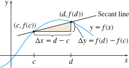
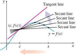
Consider the graph of the function \(y=f( x) \) shown in Figure 3. The line connecting the two points \(( c, f( c) ) \) and \(( d, f( d) ) \) on the graph of \(f\) is a secant line and its slope is \[ m_{\sec }=\dfrac{f( d) -f( c) }{d-c} \qquad d\neq c \]
Figure 4 shows there are many secant lines passing through the point \(( c, f(c)).\) If \((x,f(x))\) is any point on the graph of \(f\) with \(x\neq c\), then as the number \(x\) moves closer to \(c\), the point \((x, f(x)) \) moves along the graph of \(f\) and approaches the point \((c, f(c))\). Suppose, as the points \((x, f(x))\) get closer to the point \((c, f( c))\), the associated secant lines approach a line. Then this line is the tangent line to the graph of \(f\) at \(x=c.\) Also, the slope \(m_{\sec }\) of the secant lines approaches the slope \(m_{\tan }\) of the tangent line.
Since the slope of the secant line connecting \((c,f(c))\) and \((x,f(x) ) \) is \[ \bbox[5px, border:1px solid black, #F9F7ED] { m_{\sec }=\dfrac{f( x) -f( c) }{x-c}=\dfrac{\Delta y}{\Delta x}\qquad x\neq c } \]
the slope \(m_{\tan }\) of the tangent line is \[\bbox[5px, border:1px solid black, #F9F7ED] { m_{\tan }=\lim\limits_{x\rightarrow c}\dfrac{f( x) -f( c) }{x-c}} \]
provided the limit exists.
148
spanDEFINITIONspan Tangent Line
The tangent line to the graph of \(f\) at a point \(P\) is the line containing the point \(P=\left( c,f( c) \right)\) and having the slope \[\bbox[5px, border:1px solid black, #F9F7ED] { m_{\tan }=\lim\limits_{x\rightarrow c}\dfrac{f( x) -f( c) }{x-c}}\tag{2} \]
provided the limit exists.*
*It is possible for the limit in (2) not to exist. The geometric significance of this is discussed in the next section.
The limit in equation (1) that defines instantaneous velocity and the limit in equation (2) that defines the slope of the tangent line occur so frequently that they are given a special notation \(f^\prime (c) \), read, “\(f\) prime of \(c,\)" and called prime notation: \[\bbox[5px, border:1px solid black, #F9F7ED]{ f^\prime ( c) =\lim\limits_{x\rightarrow c}\dfrac{f( x) -f( c) }{x-c}}\tag{3} \]
THEOREM Equation of a Tangent Line
If \(m_{\tan }\) exists, then an equation of the tangent line to the graph of \(f\) at the point \(P=( c, f( c) ) \) is \[\bbox[5px, border:1px solid black, #F9F7ED]{ y-f(c)=f^\prime ( c) (x-c) \ } \]

Finding an Equation of the Tangent Line to the Graph of \(f(x) =x^{2}\)
- Find the slope of the tangent line to the graph of \(f(x) =x^{2}\) at \(c=1\) and at \(c=\) \(-2\).
- Use the results from (a) to find an equation of the tangent lines when \(c=1\) and \(c=-2\).
- Graph \(f\) and the two tangent lines on the same set of axes.
Solution
(a) At \(c=1\), the slope of the tangent line is \[ \begin{eqnarray*} f^\prime (1) &=&\lim\limits_{x\rightarrow 1}\dfrac{f(x) -f(1) }{x-1} \underset{\underset{\color{#0066A7}{f( x) =x^{2}}}{\color{#0066A7}{\uparrow }}}{=} \lim\limits_{x\rightarrow 1}\dfrac{x^{2}-1}{x-1} =\lim\limits_{x\rightarrow 1}\dfrac{( x-1) ( x+1) }{x-1}=\lim\limits_{x\rightarrow 1}( x+1) =2 \end{eqnarray*} \]
At \(c=-2\), the slope of the tangent line is \begin{eqnarray*} f^\prime ( -2) &=&\lim\limits_{x\rightarrow -2}\dfrac{ f( x) -f( -2) }{x-(-2)}=\lim\limits_{x\rightarrow -2} \dfrac{x^{2}-( -2) ^{2}}{x+2}=\lim\limits_{x\rightarrow -2}\dfrac{ x^{2}-4}{x+2}\\[11pt] &=&\lim\limits_{x\rightarrow -2}( x-2) =-4 \end{eqnarray*}
NEED TO REVIEW?
The point-slope form of a line is discussed in Appendix A.3, p. A-18.
(b) We use the results from (a) and the point-slope form of an equation of a line to obtain equations of the tangent lines. An equation of the tangent line containing the point \((1, f(1)) =(1,1) \) is \begin{eqnarray*} \begin{array}{rl@{\qquad}l} y-f(1) &= f^\prime (1) ( x-1) & {\color{#0066A7}{\hbox{Point-slope form of an equation of the tangent line.}}}\\[5pt] y-1 &= 2( x-1) & {\color{#0066A7}{\hbox{\(f(1) = 1;\quad f^\prime(1) =2.\)}}} \\[5pt] y &= 2x-1 & {\color{#0066A7}{\hbox{Simplify.}}} \end{array} \end{eqnarray*}
149
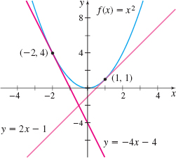
An equation of the tangent line containing the point \(( -2, f( -2)) =(-2,4) \) is \begin{eqnarray*} \begin{array}{rl@{\qquad}l} y-f( -2) &= f^\prime ( -2) [x-( -2)] \\[5pt] y-4 &=-4\cdot (x+2) & {\color{#0066A7}{\hbox{\(f(-2) = 4; \quad f^\prime (-2) =-4\)}}} \\[5pt] y &=-4x-4 \end{array} \end{eqnarray*}
(c) The graph of \(f\) and the two tangent lines are shown in Figure 5.
NOW WORK
Problem 17.
Velocity and the slope of a tangent line are each examples of the rate of change of a function.
3 Find the Rate of Change of a Function
Recall that the average rate of change of a function \(y=f( x) \) over the interval from \(c\) to \(x\) is given by \[\bbox[5px, border:1px solid black, #F9F7ED] { \hbox{Average rate of change} = \dfrac{f(x)-f( c) }{x-c} \qquad x\neq c } \]
spanDEFINITIONspan Instantaneous Rate of Change
The instantaneous rate of change of \(f\) at \(c\) is the limit as \(x\) approaches \(c\) of the average rate of change. Symbolically, the instantaneous rate of change of \(f\) at \(c\) is \[\bbox[5px, border:1px solid black, #F9F7ED] { \lim\limits_{x\rightarrow c}\dfrac{f( x) -f( c) }{x-c}} \]
provided the limit exists.
The expression “instantaneous rate of change” is often shortened to rate of change. Using prime notation, the rate of change of \(f\) at \(c\) is \(f^\prime ( c) =\ \lim\limits_{x\rightarrow c} \dfrac{f( x) -f( c) }{x-c}\) .
Finding the Rate of Change of \(f( x) =x^{2}-5x\)
Find the rate of change of the function \(f( x) =x^{2}-5x\) at:
- \(c=2\)
- any real number \(c\)
Solution (a) For \(c=2,\) \[ f( x) =x^{2}-5x \qquad \hbox{and} \qquad f(2) =2^{2}-5\cdot 2=-6 \]
The rate of change of \(f\) at \(c=2\) is \[ \begin{eqnarray*} f^\prime (2) &=& \lim\limits_{x\rightarrow 2}\dfrac{f( x) -f(2) }{x-2}=\lim\limits_{x\rightarrow 2}\dfrac{( x^{2}-5x) -( -6) }{x-2}=\lim\limits_{x\rightarrow 2}\dfrac{ x^{2}-5x+6}{x-2}\\[5pt] &=&\lim\limits_{x\rightarrow 2}\dfrac{( x-2) ( x-3) }{x-2}=\lim\limits_{x\rightarrow 2}\left( x-3\right) =-1 \end{eqnarray*} \]
(b) If \(c\) is any real number, then \(f( c) =c^{2}-5c\), and the rate of change of \(f\) at \(c\) is \[ \begin{eqnarray*} f^\prime ( c) &=&\lim\limits_{x\rightarrow c}\dfrac{f( x) -f( c) }{x-c}=\lim\limits_{x\rightarrow c}\dfrac{( x^{2}-5x) -( c^{2}-5c) }{x-c}=\lim\limits_{x\rightarrow c} \dfrac{( x^{2}-c^{2}) -5( x-c) }{x-c} \\[5pt] \notag &=&\lim\limits_{x\rightarrow c}\dfrac{( x-c) ( x+c) -5( x-c) }{x-c}=\lim\limits_{x\rightarrow c} \dfrac{( x-c) ( x+c-5) }{x-c}=\lim\limits_{x\rightarrow c} ( x+c-5) \\[3pt] &=&2c-5 \end{eqnarray*} \]
NOW WORK
Problem 25.
150
Finding the Rate of Change in a Biology Experiment
In a metabolic experiment, the mass \(M\) of glucose decreases according to the function \[ M(t) = 4.5-0.03t^{2} \]
where \(M\) is measured in grams (g) and \(t\) is the time in hours (h). Find the reaction rate \(M^\prime(t) at t=1h\).
Solution The reaction rate at \(t=1\) is \(M^\prime\) (1). \[ \begin{eqnarray*} M^\prime (1) &=&\lim\limits_{t\rightarrow 1}\dfrac{M( t) -M(1) }{t-1}=\lim\limits_{t\rightarrow 1}\dfrac{( 4.5-0.03t^{2}) -( 4.5-0.03) }{t-1}\\[5pt] &=&\lim\limits_{t\rightarrow 1}\dfrac{-0.03t^{2}+0.03}{t-1} =\lim\limits_{t\rightarrow 1}\dfrac{( -0.03) ( t^{2}-1 ) }{t-1}=\lim\limits_{t\rightarrow 1}\dfrac{( -0.03) ( t-1) ( t+1) }{t-1}\\[5pt] &=&( -0.03) (2) =-0.06\\[-20pt] \end{eqnarray*} \]
The reaction rate at \(t=1\) h is \(-0.06\)g/h. That is, the mass \(M\) of glucose at \(t=1\) h is decreasing at the rate of 0.06g/h.
NOW WORK
Problem 43.
4 Find the Derivative of a Function at a Number
Velocity, slope of a tangent line, and rate of change of a function are all found using the same limit, \[ f^\prime ( c) =\lim\limits_{x\rightarrow c}\dfrac{f( x) -f( c) }{x-c}\ \]
The common underlying idea is the mathematical concept of derivative.
spanDEFINITIONspan Derivative of a Function at a Number
If \(y=f( x) \) is a function and \(c\) is in the domain of \(f\) , then the derivative of \(f\) at \(c\), denoted by \(f^\prime ( c) \), is the number \[\bbox[5px, border:1px solid black, #F9F7ED]{ f^\prime (c) =\lim\limits_{x\rightarrow c}\dfrac{f( x) -f( c) }{x-c}} \]
provided this limit exists.
So far, we have given three interpretations of the derivative:
- Physical interpretation: When the distance \(s\) at time \(t\) of an object in rectilinear motion is given by the function \(s=f( t) \), the derivative \(f^\prime ( t_{0}) \) is the velocity of the object at time \(t_{0}\).
- Geometric interpretation: If \(y=f( x) ,\) the derivative \(f^\prime (c) \) is the slope of the tangent line to the graph of \(f\) at the point \((c, f(c)) .\)
- Rate of change of a function interpretation: If \(y=f( x) ,\) the derivative \(f^\prime ( c) \) is the rate of change of \(f\) at \(c.\)
Finding the Derivative of a Function at a Number
Find the derivative of \(f(x) =2x^{3}-5x\) at \(x=1\). That is, find \(f^\prime (1) \).
Solution Using the definition of a derivative, we have \[ \begin{array}{@{\hspace*{-4pc}}rcl} f^\prime (1) &=&\lim\limits_{x\rightarrow 1}\dfrac{f( x) -f(1) }{x-1}=\lim\limits_{x\rightarrow 1}\dfrac{( 2x^{3}-5x) -( -3) }{x-1}=\lim\limits_{x\rightarrow 1}\dfrac{ 2x^{3}-5x+3}{x-1} \quad {\color{#0066A7}{\hbox{\(f(1) =2-5=-3\)}}} \\ &=&\lim\limits_{x\rightarrow 1}\dfrac{( x-1) ( 2x^{2}+2x-3) }{x-1}=\lim\limits_{x\rightarrow 1}(2x^{2}+2x-3) =2+2-3=1 \end{array} \]
NOW WORK
Problem 27.
151
Finding an Equation of a Tangent Line
- Find the derivative of \(f( x) =\sqrt{2x}\) at \(x=8.\)
- Use the derivative \(f^\prime ( 8)\) to find the equation of the tangent line to the graph of \(f\) at the point (8,4).
Solution (a) The derivative of \(f\) at \(8\) is \[ \begin{eqnarray*} f^\prime (8) &=& \lim\limits_{x\rightarrow 8}\dfrac{f( x) -f( 8) }{x-8} {=} \lim\limits_{x\rightarrow 8}\dfrac{ \sqrt{2x}-4}{x-8} {=} \lim\limits_{x\rightarrow 8}\dfrac{( \sqrt{2x}-4) ( \sqrt{2x}+4) }{( x-8) ( \sqrt{2x}+4) }\\[-6.4pt] &&\hspace{4.0pc}\underset{\color{#0066A7}{f(8) =\sqrt{2\cdot 8} = 4}}{\color{#0066A7}{\uparrow}}\hspace{1.1pc} \underset{\underset{\color{#0066A7}{\scriptsize \hspace{0.4pc}\hbox{the numerator.}}}{\color{#0066A7}{\scriptsize \hbox{Rationalize}}}}{\color{#0066A7}{\uparrow}}\\ &=& \lim\limits_{x\rightarrow 8}\dfrac{2x-16}{( x-8) ( \sqrt{ 2x}+4) } =\lim\limits_{x\rightarrow 8}\dfrac{2( x-8) }{ ( x-8) ( \sqrt{2x}+4) }=\lim\limits_{x\rightarrow 8} \dfrac{2}{\sqrt{2x}+4}=\dfrac{1}{4} \end{eqnarray*} \]
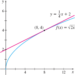
(b) The slope of the tangent line to the graph of \(f\) at the point \((8,4) \) is \(f^\prime (8) =\dfrac{1}{4}.\) Using the point-slope form of a line, we get \[ \begin{eqnarray*} \begin{array}{rl@{\qquad}l} y-f( 8) &= f^\prime ( 8) ( x-8) & {\color{#0066A7}{\hbox{\({y-y}_{1}=m ( {x-x}_{1})\)}}} \\[6pt] \notag y-4 &= \dfrac{1}{4}( x-8) & {\color{#0066A7}{\hbox{\({f}( {8}) = 4; \quad {f^\prime }(8) = \dfrac{1}{4}\)}}} \\[9pt] \notag y &= \dfrac{1}{4}x-\dfrac{1}{4}\cdot 8+4 \\[9pt] \notag y &= \dfrac{1}{4}x+2 \end{array} \end{eqnarray*} \]
The graphs of \(f\) and the tangent line to the graph of \(f\) at \((8,4)\) are shown in Figure 6.