10.6 Power Series
A power series with center \(a\) is an infinite series \[ F(x) = \sum_{n=0}^{\infty} a_n(x-a)^n = a_0 + a_1 (x-a) + a_2 (x-a)^2 + a_3(x-a)^3 + \cdots \] where \(x\) is a variable. For example, \[ \begin{equation*} F(x) = 1+(x-2)+2(x-2)^2+3(x-2)^3 +\cdots\tag{1} \end{equation*} \] is a power series with center \(a=2\).
580
A power series \(\displaystyle\sum^\infty_{n=0} a_n(x-a)^n\) converges for some values of \(x\) and may diverge for others. For example, if we set \(x=\tfrac94\) in the power series of Eq. (1), we obtain an infinite series that converges by the Ratio Test: \[ \begin{align*} F\left(\dfrac94\right) &= 1+\left(\dfrac94-2\right)+2\left(\dfrac94-2\right)^2+3\left(\dfrac94-2\right)^3 +\cdots\\ &= 1 + \left(\dfrac14\right)+2\left(\dfrac14\right)^2+3\left(\dfrac14\right)^3+\cdots \end{align*} \]
Many functions that arise in applications can be represented as power series. This includes not only the familiar trigonometric, exponential, logarithm, and root functions, but also the host of “special functions” of physics and engineering such as Bessel functions and elliptic functions.
On the other hand, the power series in Eq. (1) diverges for \(x=3\): \[ \begin{align*} F(3) &= 1+(3-2)+2(3-2)^2+3(3-2)^3 +\cdots\\ &= 1+1+2+3+\cdots \end{align*} \]
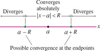
There is a surprisingly simple way to describe the set of values \(x\) at which a power series \(F(x)\) converges. According to our next theorem, either \(F(x)\) converges absolutely for all values of \(x\) or there is a radius of convergence \(R\) such that \[ \boxed{\bbox[#FAF8ED,5pt]{\textrm{\(F(x)\) converges absolutely when \(|x-a|<R\) and diverges when \(|x-a|>R\).}}} \]
This means that \(F(x)\) converges for \(x\) in an interval of convergence consisting of the open interval \((a-R, a+R)\) and possibly one or both of the endpoints \(a-R\) and \(a+R\) (Figure 10.23). Note that \(F(x)\) automatically converges at \(x=a\) because \[ F(a) = a_0 + a_1 (a-a) + a_2(a-a)^2 + a_3(a-a)^3 + \cdots = a_0 \] We set \(R=0\) if \(F(x)\) converges only for \(x=a\), and we set \(R=\infty\) if \(F(x)\) converges for all values of \(x\).
THEOREM 1 Radius of Convergence
Every power series \[F(x) = \sum_{n=0}^{\infty} a_n(x-a)^n\] has a radius of convergence \(R\), which is either a nonnegative number (\(R\ge 0\)) or infinity (\(R=\infty\)). If \(R\) is finite, \(F(x)\) converges absolutely when \(|x-a|<R\) and diverges when \(|x-a|>R\). If \(R=\infty\), then \(F(x)\) converges absolutely for all \(x\).
Proof
We assume that \(a=0\) to simplify the notation. If \(F(x)\) converges only at \(x=0\), then \(R=0\). Otherwise, \(F(x)\) converges for some nonzero value \(x=B\). We claim that \(F(x)\) must then converge absolutely for all \(\left|x\right|<|B|\). To prove this, note that because \({\displaystyle F(B) = \sum_{n=0}^\infty a_nB^n}\) converges, the general term \(a_nB^n\) tends to zero. In particular, there exists \(M>0\) such that \(|a_nB^n|<M\) for all \(n\). Therefore,
581
\[ \sum_{n=0}^\infty \left|a_nx^n \right| = \sum_{n=0}^\infty |a_nB^n|\,\left|\frac{x}{B}\right|^n < M\sum_{n=0}^\infty \left|\frac{x}{B}\right|^n \] If \(\left|x\right|<|B|\), then \(|x/B|<1\) and the series on the right is a convergent geometric series. By the Comparison Test, the series on the left also converges. This proves that \(F(x)\) converges absolutely if \(\left|x\right| < |B|\).
Now let \(S\) be the set of numbers \(x\) such that \(F(x)\) converges. Then \(S\) contains 0, and we have shown that if \(S\) contains a number \(B \neq 0\), then \(S\) contains the open interval \((-|B|,|B|)\). If \(S\) is bounded, then \(S\) has a least upper bound \(L > 0\) (see marginal note). In this case, there exist numbers \(B \in S\) smaller than but arbitrarily close to \(L\), and thus \(S\) contains \((-B, B)\) for all \(0 < B < L\). It follows that \(S\) contains the open interval \((-L, L)\). The set \(S\) cannot contain any number \(x\) with \(\left|x\right| > L\), but \(S\) may contain one or both of the endpoints \(x = \pm L\). So in this case, \(F(x)\) has radius of convergence \(R=L\). If \(S\) is not bounded, then \(S\) contains intervals \((-B, B)\) for \(B\) arbitrarily large. In this case, \(S\) is the entire real line R, and the radius of convergence is \(R=\infty\).
Least Upper Bound Property: If \(S\) is a set of real numbers with an upper bound \(M\) (that is, \(x \leq M\) for all \(x \in S\)), then \(S\) has a least upper bound \(L\). See Appendix B.
From Theorem 1, we see that there are two steps in determining the interval of convergence of \(F(x)\):
Step 1. Find the radius of convergence \(R\) (using the Ratio Test, in most cases).
Step 2. Check convergence at the endpoints (if \(R\ne 0\) or \(\infty\)).
EXAMPLE 1 Using the Ratio Test
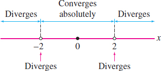
Where does F(x)=\(\displaystyle\sum^\infty_{n=0} \dfrac{x^n}{2^n}\) converge?
Solution
Step 1.Find the radius of convergence.
Let \(a_n = \dfrac{x^n}{2^n}\) and compute the ratio \(\rho\) of the Ratio Test: \[ \rho = \lim_{n\to\infty}\left|\frac{a_{n+1}}{a_n}\right| = \lim_{n\to\infty}\left|\frac{x^{n+1}}{2^{n+1}} \right| \cdot \left| \frac{2^n}{x^n} \right| = \lim_{n\to\infty} \frac{1}{2}\left|x\right| = \frac{1}{2}\left|x\right| \] We find that \[ \rho<1\qquad {if}\quad \frac12 \left|x\right|<1, \qquad{\text{that is, if}}\quad \left|x\right|<2 \] Thus \(F(x)\) converges if \(\left|x\right| < 2\). Similarly, \(\rho > 1\) if \(\tfrac{1}{2} \left|x\right| >1\), or \(\left|x\right| >2\). Thus \(F(x)\) diverges if \(\left|x\right| >2\). Therefore, the radius of convergence is \(R=2\).
Step 2. Check the endpoints.
The Ratio Test is inconclusive for \(x=\pm 2\), so we must check these cases directly: \[ \begin{align*} F(2)&=\sum_{n=0}^{\infty} \dfrac{2^n}{2^n} = 1 + 1 + 1 + 1 +1 +1 \cdots \\ F(-2)&=\sum_{n=0}^{\infty} \dfrac{(-2)^n}{2^n} = 1 - 1 + 1 - 1 +1 -1 \cdots \end{align*} \] Both series diverge. We conclude that \(F(x)\) converges only for \(\left|x\right| < 2\) (Figure 10.24).
582
EXAMPLE 2
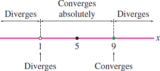
Where does \(\displaystyle F(x)=\sum\limits_{n=1}^\infty \frac{(-1)^n}{4^n\,n} (x-5)^n\) converge?
Solution We compute \(\rho\) with \(\displaystyle a_n = \frac{(-1)^n}{4^n\,n}(x-5)^n\): \[ \begin{align*} \rho = \lim_{n\to\infty}\left|\frac{a_{n+1}}{a_n}\right| &= \lim_{n\to\infty} \left| \frac{(x-5)^{n+1}}{4^{n+1}(n+1)}\,\frac{4^n n}{(x-5)^n} \right|\\ &=|x-5| \lim_{n\to\infty} \left| \frac{n}{4(n+1)} \right|\\&= \frac14 |x-5| \end{align*} \] We find that \[ \rho<1 \qquad \textrm{if}\quad \frac14|x-5|<1,\qquad\textrm{that is, if}\quad |x-5|<4 \]
Thus \(F(x)\) converges absolutely on the open interval \((1,9)\) of radius \(4\) with center \(a=5\). In other words, the radius of convergence is \(R=4\). Next, we check the endpoints: \[ \begin{align*} &x=9{:}&\quad &\sum_{n=1}^\infty \frac{(-1)^n}{4^nn} (9-5)^n = \sum_{n=1}^\infty \frac{(-1)^n}{n}&\quad&\textrm{converges (Leibniz Test)}\\ &x=1{:}&\quad &\sum_{n=1}^\infty \frac{(-1)^n}{4^nn} (-4)^n = \sum_{n=1}^\infty \frac{1}{n}&\quad&\textrm{diverges (harmonic series)} \end{align*} \] We conclude that \(F(x)\) converges for \(x\) in the half-open interval \((1,9]\) shown in Figure 10.25.
Some power series contain only even powers or only odd powers of \(x\). The Ratio Test can still be used to find the radius of convergence.
Question 10.13 Power Series Progress Check Question 1
What is the radius of convergence of the series \( \displaystyle \sum_{n=1}^\infty \frac{x^n}{n2^n}\) ?
Question 10.14 Power Series Progress Check Question 2
What is the interval of convergence of \( \displaystyle \sum_{n=1}^\infty \frac{x^n}{n2^n}\) ?
| A. |
| B. |
| C. |
| D. |
| E. |
EXAMPLE 3 An Even Power Series
Where does \(\displaystyle\sum^\infty_{n=0} \frac{x^{2n}}{(2n)!}\) converge?
Solution Although this power series has only even powers of \(x\), we can still apply the Ratio Test with \(a_n = {x^{2n}}/{(2n)!}\). We have \[a_{n+1} = \frac{x^{2(n+1)}}{(2(n+1))!}=\frac{x^{2n+2}}{(2n+2)!}\] Furthermore, \((2n+2)! = (2n+ 2)(2n +1)(2n)!\), so \[ \begin{align*} \rho =\lim_{n\to\infty}\left|\frac{a_{n+1}}{a_n}\right| = \lim_{n\to\infty} \frac{x^{2n+2}}{(2n+2)!}\frac{(2n)!}{x^{2n}} = \left|x\right|^2\lim_{n\to\infty} \frac1{(2n+2)(2n+1)} =0 \end{align*} \] Thus \(\rho = 0\) for all \(x\), and \(F(x)\) converges for all \(x\). The radius of convergence is \(R=\infty\).
Question 10.15 Power Series Progress Check Question 3
Find the radius and interval of convergence of \(\displaystyle\sum^\infty_{n=0} \frac{x^{2n+1}}{(2n+1)!}\)
| A. |
| B. |
| C. |
| D. |
| E. |
| F. |
583
Geometric series are important examples of power series. Recall the formula \({\displaystyle\sum\limits_{n=0}^\infty r^n= 1/({1-r})}\), valid for \(|r|<1\). Writing \(x\) in place of \(r\), we obtain a power series expansion with radius of convergence \(R=1\): \[ \begin{equation*} \boxed{\bbox[#FAF8ED,5pt]{\frac{1}{1-x} = \sum\limits_{n=0}^\infty\,x^n\qquad\textrm{for \(\left|x\right| < 1\)}}}\tag{2} \end{equation*} \]
When a function \(f(x)\) is represented by a power series on an interval \(I\), we refer to the power series expansion of \(f(x)\) on \(I\).
The next two examples show that we can modify this formula to find the power series expansions of other functions.
EXAMPLE 4 Geometric Series
Prove that \[ \frac1{1-2x}=\sum_{n=0}^\infty 2^nx^n \qquad\textrm{for \(\left|x\right|<\frac12\)} \]
Solution Substitute \(2x\) for \(x\) in Eq. (2): \[ \begin{equation*} \frac{1}{1-2x} = \sum_{n=0}^\infty (2x)^n = \sum_{n=0}^\infty 2^nx^n\tag{3} \end{equation*} \]
Expansion (2) is valid for \(\left|x\right|<1\), so Eq. (3) is valid for \(|2x|<1\), or \(\left|x\right|<\frac12\).
EXAMPLE 5
Find a power series expansion with center \(a=0\) for \[f(x)=\frac1{2+x^2}\] and find the interval of convergence.
Solution We need to rewrite \(f(x)\) so we can use Eq. (2). We have \[ \frac1{2+x^2} = \frac12\,\left(\frac1{ 1 + \frac12x^2}\right) = \frac12 \left(\frac1{1 - \big(-\frac12x^2\big)}\right)=\frac12\left(\frac{1}{1-u}\right) \] where \(u =-\tfrac12 x^2\). Now substitute \(u = -\frac12x^2\) for \(x\) in Eq. (2) to obtain \[ \begin{align*} f(x)=\frac1{2+x^2} &= \frac12\sum_{n=0}^\infty \biggl(-\frac{x^2}2\biggr)^n\\ & = \sum_{n=0}^\infty \frac{(-1)^nx^{2n}}{2^{n+1}} \end{align*} \] This expansion is valid if \(|{-x^2}/{2}|<1\), or \(\left|x\right|<\sqrt{2}\). The interval of convergence is \((-\sqrt{2},\sqrt{2})\).
Our next theorem tells us that within the interval of convergence, we can treat a power series as though it were a polynomial; that is, we can differentiate and integrate term by term.
584
The proof of Theorem 2 is somewhat technical and is omitted. See Exercise 66 for a proof that \(F(x)\) is continuous.
THEOREM 2 Term-by-Term Differentiation and Integration
Assume that \[ F(x) = \sum_{n=0}^{\infty} a_n(x-a)^n \] has radius of convergence \(R>0\). Then \(F(x)\) is differentiable on \((a-R, a+R)\) [or for all \(x\) if \(R=\infty\)]. Furthermore, we can integrate and differentiate term by term. For \(x \in (a-R, a+R)\), \[ \begin{align*} F'(x) &= \sum_{n=1}^\infty\, na_n(x-a)^{n-1}\\ \int F(x)\, dx &= C+\sum_{n=0}^\infty \frac{a_n}{n+1}(x-a)^{n+1}\qquad (\textrm{\(C\) any constant}) \end{align*} \] These series have the same radius of convergence \(R\).
EXAMPLE 6 Differentiating a Power Series
Prove that for \(-1 <x < 1\), \[ \frac1{(1-x)^2} = 1+2x+3x^2+4x^3+5x^4+\cdots \]
Solution The geometric series has radius of convergence \(R=1\): \[\frac{1}{1-x} =1+x+x^2+x^3+x^4 +\cdots \] By Theorem 2, we can differentiate term by term for \(\left|x\right|<1\) to obtain \[ \begin{align*} \frac{d}{dx} \,\Big(\frac{1}{1-x}\Big) &= \frac{d}{dx} (1+x+x^2+x^3+x^4 +\cdots )\notag \\ \frac1{(1-x)^2} &= 1+2x+3x^2+4x^3+5x^4+\cdots \end{align*} \]
Theorem 2 is a powerful tool in the study of power series.
EXAMPLE 7 Power Series for Arctangent
Prove that for \(-1 <x < 1\), \[ \begin{align*} \tan^{-1}x =\sum_{n=0}^\infty \frac{(-1)^{n}x^{2n+1}}{2n+1} = x-\frac{x^3}3+\frac{x^5}5-\frac{x^7}7+\cdots\tag{4} \end{align*} \]
Solution Recall that \(\tan^{-1}x\) is an antiderivative of \((1+x^2)^{-1}\). We obtain a power series expansion of this antiderivative by substituting \(-x^2\) for \(x\) in the geometric series of Eq.(2): \[ \frac{1}{1+x^2}= 1-x^2+x^4-x^6+\cdots \]
This expansion is valid for \(|x^2|<1\)–that is, for \(\left|x\right|<1\). By Theorem 2, we can integrate series term by term. The resulting expansion is also valid for \(\left|x\right|<1\): \[ \begin{align*} \tan^{-1}x &= \int\frac{dx}{1+x^2} = \int (1-x^2+x^4-x^6+\cdots )\, dx\\ & = C+x - \frac{x^3}3+\frac{x^5}5-\frac{x^7}7+\cdots \end{align*} \]
Setting \(x=0\), we obtain \(C = \tan^{-1}0 =0\). Thus Eq. (4) is valid for \(-1 < x < 1\).
585
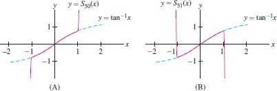
GRAPHICAL INSIGHT
Let’s examine the expansion of the previous example graphically. The partial sums of the power series for \(f(x) = \tan^{-1}x\) are \[ S_N(x) = x - \frac{x^3}3+\frac{x^5}5-\frac{x^7}7 + \cdots + (-1)^N \frac{x^{2N+1}}{2N+1} \]
For large \(N\) we can expect \(S_N(x)\) to provide a good approximation to \(f(x) = \tan^{-1}x\) on the interval \((-1,1)\), where the power series expansion is valid. Figure 10.26 confirms this expectation: The graphs of \(S_{50}(x)\) and \(S_{51}(x)\) are nearly indistinguishable from the graph of \(\tan^{-1}x\) on \((-1,1)\). Thus we may use the partial sums to approximate the arctangent. For example, \(\tan^{-1}~(0.3)\) is approximated by \[ S_4(0.3) = 0.3-\frac{(0.3)^3}3+\frac{(0.3)^5}5 - \frac{(0.3)^7}7+ \frac{(0.3)^9}9 \approx 0.2914569 \]
Since the power series is an alternating series, the error is less than the first omitted term: \[ |{\tan^{-1}(0.3)-S_4(0.3)}| < \frac{(0.3)^{11}}{11} \approx 1.61 \times 10^{-7} \] The situation changes drastically in the region \(\left|x\right|>1\), where the power series diverges and the partial sums \(S_N(x)\) deviate sharply from \(\tan^{-1}x\).
Power Series Solutions of Differential Equations
Power series are a basic tool in the study of differential equations. To illustrate, consider the differential equation with initial condition \[ y'=y,\qquad y(0) = 1 \] We know that \(f(x)=e^x\) is the unique solution, but let’s try to find a power series that satisfies this initial value problem. We have \[ \begin{align*} F(x) &= \sum_{n=0}^\infty a_nx^n = a_0+a_1x+a_2x^2+a_3x^3+\cdots\\ F'(x) &=\sum_{n=0}^\infty na_nx^{n-1} = a_1+2a_2x+3a_3x^2+4a_4x^3+\cdots \end{align*} \] Therefore, \(F'(x) =F(x)\) if \[ a_0=a_1,\quad a_1=2a_2,\quad a_2=3a_3,\quad a_3=4a_4,\quad\dots \]
586
In other words, \(F'(x) = F(x)\) if \(a_{n-1}=na_n\), or \[ \boxed{\bbox[#FAF8ED,5pt]{ a_{n} = \frac{a_{n-1}}{n}}} \] An equation of this type is called a recursion relation. It enables us to determine all of the coefficients \(a_n\) successively from the first coefficient \(a_0\), which may be chosen arbitrarily. For example, \[ \begin{alignat*}{2} n&=1{:}&\qquad &a_1 = \frac{a_0}1\\ n&=2{:}&\qquad &a_2 =\frac{a_1}2=\frac{a_0}{2\cdot 1}=\frac{a_0}{2!}\\ n&=3{:}&\qquad &a_3=\frac{a_2}3=\frac{a_1}{3\cdot 2}=\frac{a_0}{3\cdot 2\cdot 1}=\frac{a_0}{3!} \end{alignat*} \] To obtain a general formula for \(a_n\), apply the recursion relation \(n\) times: \[ a_n=\frac{a_{n-1}}n=\frac{a_{n-2}}{n(n-1)} = \frac{a_{n-3}}{n(n-1)(n-2)} = \cdots = \frac{a_0}{n!} \] We conclude that \[F(x)=a_0\sum_{n=0}^\infty \frac{x^n}{n!}\] In Example 3, we showed that this power series has radius of convergence \(R=\infty\), so \(y=F(x)\) satisfies \(y'=y\) for all \(x\). Moreover, \(F(0) = a_0\), so the initial condition \(y(0)=1\) is satisfied with \(a_0=1\).
What we have shown is that \(f(x)=e^x\) and \(F(x)\) with \(a_0 =1\) are both solutions of the initial value problem. They must be equal because the solution is unique. This proves that for all \(x\), \[ \begin{equation*} \boxed{\bbox[#FAF8ED,5pt]{ e^x = \sum\limits_{n=0}^\infty \frac{x^n}{n!} = 1 + x + \frac{x^2}{2!}+\frac{x^3}{3!}+\frac{x^4}{4!}+ \cdots}} \end{equation*} \]
In this example, we knew in advance that \(y=e^x\) is a solution of \(y'=y\), but suppose we are given a differential equation whose solution is unknown. We can try to find a solution in the form of a power series \({\displaystyle F(x)=\sum_{n=0}^\infty a_nx^n }\). In favorable cases, the differential equation leads to a recursion relation that enables us to determine the coefficients \(a_n\).
The solution in Example 8 is called the “Bessel function of order 1.” The Bessel function of order \(n\) is a solution of \[ x^2y''+xy'+(x^2-n^2)y=0 \] These functions have applications in many areas of physics and engineering.
EXAMPLE 8
Find a power series solution to the initial value problem \[ \begin{equation*} x^2y''+xy'+(x^2-1)y=0,\qquad y'(0) = 1 \tag{5} \end{equation*} \]
Solution Assume that Eq.(5) has a power series solution \(F(x)= \sum\limits_{n=0}^\infty a_nx^n\). Then \[ \begin{align*} y'=F'(x) &= \sum_{n=0}^\infty na_nx^{n-1} = a_1 + 2a_2 x + 3a_3 x^2 + \cdots\\ y''=F''(x) &= \sum_{n=0}^\infty n(n-1)a_nx^{n-2} = 2a_2 + 6a_3 x + 12a_4 x^2 + \cdots \end{align*} \]
587
Now substitute the series for \(y\), \(y'\), and \(y''\) into the differential equation (5) to determine the recursion relation satisfied by the coefficients \(a_n\): \[ \begin{eqnarray*} &&x^2y''+xy'+(x^2-1)y \\ &&\qquad = x^2\sum_{n=0}^\infty n(n-1)a_nx^{n-2}+x\sum_{n=0}^\infty na_nx^{n-1} +(x^2-1)\sum_{n=0}^\infty a_nx^n\\ &&\qquad= \sum_{n=0}^\infty n(n-1)a_nx^n+ \sum_{n=0}^\infty na_nx^n-\sum_{n=0}^\infty a_nx^n+ \sum_{n=0}^\infty a_nx^{n+2}\\ &&\qquad= \sum_{n=0}^\infty (n^2-1)a_nx^n + \sum_{n=2}^\infty a_{n-2}x^{n}=0\tag{6} \end{eqnarray*} \]
In Eq.(6), we combine the first three series into a single series using \[ n(n-1)+n-1=n^2-1 \] and we shift the fourth series to begin at \(n=2\) rather than \(n=0\).
The differential equation is satisfied if \[ \sum_{n=0}^\infty (n^2-1)a_nx^n = -\sum_{n=2}^\infty a_{n-2}x^n \]
The first few terms on each side of this equation are \[ -a_0+0\cdot x + 3a_2x^2+8a_3x^3 + 15a_4x^4 + \cdots = 0+0\cdot x -a_0x^2-a_1x^3-a_2x^4-\cdots \]
Matching up the coefficients of \(x^n\), we find that \[ \begin{align*} -a_0 = 0,\qquad 3a_2 = -a_0,\qquad 8a_3 = -a_1,\qquad 15a_4 = -a_2\tag{7} \end{align*} \]
In general, \((n^2-1)a_n = -a_{n-2}\), and this yields the recursion relation \[ \boxed{\bbox[#FAF8ED,5pt]{ a_n = -\frac{a_{n-2}}{n^2-1}\qquad \textrm{for \(n\ge 2\)}}}\tag {8} \]
Note that \(a_0=0\) by Eq. (7). The recursion relation forces all of the even coefficients \(a_2\), \(a_4\), \(a_6, \dots\) to be zero: \[ \textrm{\(a_2=\frac{a_0}{2^2-1}\) so \(a_2=0\), and then \(a_4=\frac{a_2}{4^2-1}=0\) so \(a_4=0\), etc.} \]
As for the odd coefficients, \(a_1\) may be chosen arbitrarily. Because \(F'(0) = a_1\), we set \(a_1=1\) to obtain a solution \(y = F(x)\) satisfying \(F'(0)=1\). Now apply Eq. (8): \[ \begin{alignat*}{2} n&=3{:}\qquad& a_3 &= -\frac{a_1}{3^2-1}= -\frac{1}{3^2-1}\\ n&=5{:} \qquad&a_5 &= -\frac{a_3}{5^2-1} = \frac{1}{(5^2-1)(3^2-1)}\\ n&=7{:} \qquad&a_7 &= -\frac{a_5}{7^2-1} = -\frac{1}{(7^2-1)(3^2-1)(5^2-1)} \end{alignat*} \]
This shows the general pattern of coefficients. To express the coefficients in a compact form, let \(n=2k+1\). Then the denominator in the recursion relation (8) can be written \[ n^2-1=(2k+1)^2-1=4k^2+4k=4k(k+1) \] and \[ a_{2k+1} = - \frac{a_{2k-1}}{4k(k+1)} \]
588
Applying this recursion relation \(k\) times, we obtain the closed formula \[ a_{2k+1} = (-1)^k \left( \frac{1}{4k(k+1)}\right) \left(\frac{1}{4(k-1)k}\right)\cdots \left(\frac{1}{4(1)(2)}\right) = \frac{(-1)^k}{4^k\,k!\,(k+1)!} \]
Thus we obtain a power series representation of our solution: \[ F(x) = \sum_{k=0}^\infty\,\frac{(-1)^k}{4^kk!(k+1)!}x^{2k+1} \]
A straightforward application of the Ratio Test shows that \(F(x)\) has an infinite radius of convergence. Therefore, \(F(x)\) is a solution of the initial value problem for all \(x\).
10.6.1 Summary
- A power series is an infinite series of the form \[ F(x) = \sum_{n=0}^\infty a_n (x-a)^n \] The constant \(a\) is called the center of \(F(x)\).
- Every power series \(F(x)\) has a radius of convergence \(R\) (Figure 10.27) such that
- - \(F(x)\) converges absolutely for \(|x-a|<R\) and diverges for \(|x-a|>R\).
- - \(F(x)\) may converge or diverge at the endpoints \(a-R\) and \(a+R\).
- The interval of convergence of \(F(x)\) consists of the open interval \((a-R, a+R)\) and possibly one or both endpoints \(a-R\) and \(a+R\).
- In many cases, the Ratio Test can be used to find the radius of convergence \(R\). It is necessary to check convergence at the endpoints separately.
- If \(R > 0\), then \(F(x)\) is differentiable on \((a-R, a+R)\) and \[ F'(x) = \sum_{n=1}^\infty na_n(x - a)^{n-1},\qquad \int F(x)\, dx = C+ \sum_{n=0}^\infty \frac{a_n}{n+1}(x - a)^{n+1} \] (\(C\) is any constant). These two power series have the same radius of convergence \(R\).
- The expansion \({\displaystyle \frac{1}{1-x}=\sum_{n=0}^\infty x^n}\) is valid for \(\left|x\right|<1\). It can be used to derive expansions of other related functions by substitution, integration, or differentiation.