12.3 Vectors in Three Dimensions
This section extends the vector concepts introduced in the previous section to three-dimensional space. We begin with some introductory remarks about the three-dimensional coordinate system.
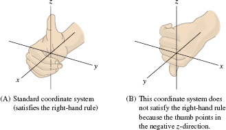
By convention, we label the axes as in Figure 12.21, where the positive sides of the axes are labeled \(x\), \(y\), and \(z\). This labeling satisfies the right-hand rule, which means that when you position your right hand so that your fingers curl from the positive \(x\)-axis toward the positive \(y\)-axis, your thumb points in the positive \(z\)-direction. The axes in Figure 12.21 are not labeled according to the right-hand rule.
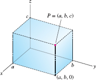
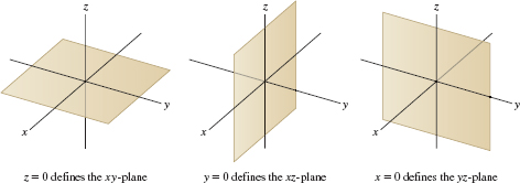
Each point in space has unique coordinates \((a,b,c)\) relative to the axes (Figure 12.22). We denote the set of all triples \((a,b,c)\) by \(\textbf{R}^3\). The coordinate planes in \(\textbf{R}^3\) are defined by setting one of the coordinates equal to zero (Figure 12.23). The \(xy\)-plane consists of the points \((a,b,0)\) and is defined by the equation \(z=0\). Similarly, \(x=0\) defines the \(yz\)-plane consisting of the points \((0,b,c)\), and \(y=0\) defines the \(xz\)-plane consisting of the points \((a,0,c)\). The coordinate planes divide \(\textbf{R}^3\) into eight octants (analogous to the four quadrants in the plane). Each octant corresponds to a possible combination of signs of the coordinates. The set of points \((a,b,c)\) with \(a,b,c gt 0\) is called the first octant.
As in two dimensions, we derive the distance formula in \(\textbf{R}^3\) from the Pythagorean Theorem.
THEOREM 1 Distance Formula in \(\textbf{R}^3\)]
The distance \(|P-Q|\) between the points \(P=(a_1,b_1,c_1)\) and \(Q=(a_2,b_2,c_2)\) is \begin{equation} |P-Q|=\sqrt{(a_2-a_1)^2+(b_2-b_1)^2+(c_2-c_1)^2}\tag{1} \end{equation}
669
First apply the distance formula in the plane to the points \(P\) and \(R\) (Figure 12.24): \[ |P-R|^2 = (a_2-a_1)^2+(b_2-b_1)^2 \]
Then observe that \(\triangle \textit{PRQ}\) is a right triangle [Figure 12.24] and use the Pythagorean Theorem: \begin{align*} |P-Q|^2 = |P-R|^2+|R-Q|^2 = (a_2-a_1)^2+(b_2-b_1)^2 +(c_2-c_1)^2 \end{align*}

The sphere of radius \(R\) with center \(Q=(a,b,c)\) consists of all points \(P=(x,y,z)\) located a distance \(R\) from \(Q\) (Figure 12.25). By the distance formula, the coordinates of \(P=(x,y,z)\) must satisfy \[ \sqrt{(x-a)^2+(y-b)^2+(z-c)^2} = R \]
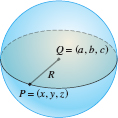
On squaring both sides, we obtain the standard equation of the sphere [Eq. (3) below].
Now consider the equation \begin{equation} (x-a)^2+(y-b)^2 = R^2 \end{equation}
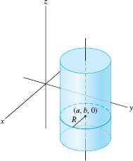
In the \(xy\)-plane, Eq. (2) defines the circle of radius \(R\) with center \((a,b)\). However, as an equation in \(\textbf{R}^3\), it defines the right circular cylinder of radius \(R\) whose central axis is the vertical line through \((a,b,0)\) (Figure 12.26). Indeed, a point \((x,y,z)\) satisfies Eq. (2) for any value of \(z\) if \((x,y)\) lies on the circle. It is usually clear from the context which of the following is intended: \begin{align*} \textrm{Circle}&=\{ (x,y): (x-a)^2+(y-b)^2=R^2\}\\ \textrm{Right circular cylinder}&=\{ (x,y,z): (x-a)^2+(y-b)^2=R^2\} \end{align*}
670
Equations of Spheres and Cylinders
An equation of the sphere in \(\textbf{R}^3\) of radius \(R\) centered at \(Q=(a,b,c)\) is \begin{equation} \label{14.vec3.sphereeq} (x-a)^2+(y-b)^2+(z-c)^2 = R^2\tag{3} \end{equation}
An equation of the right circular cylinder in \(\textbf{R}^3\) of radius \(R\) whose central axis is the vertical line through \((a,b,0)\) is \begin{equation} (x-a)^2+(y-b)^2 = R^2\tag{4} \end{equation}
EXAMPLE 1
Describe the sets of points defined by the following conditions:
- (a) (\(x^2+y^2+z^2 = 4,\quad y \ge 0\)
- (b) \((x-3)^2+(y-2)^2 = 1,\quad z\ge -1\)
Solution
- (a) The equation \(x^2+y^2+z^2 = 4\) defines a sphere of radius 2 centered at the origin. The inequality \(y\ge 0\) holds fo points lying on the positive side of the \(xz\)-plane. We obtain the right hemisphere of radius 2illustrated in Figure 12.27.
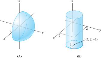 Figure 12.27: Hemisphere and upper cylinder.
 - (b) The equation \((x-3)^2+(y-2)^2 = 1\) defines a cylinder of radius 1 whose central axis is the vertical line through \((3,2,0)\). The part of the cylinder where \(z \geq -1\) is illustrated in Figure 12.27.
Vector Concepts
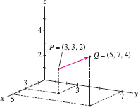
As in the plane, a vector \(\textbf{v} = \overrightarrow{PQ}\) in \(\textbf{R}^3\) is determined by an initial point \(P\) and a terminal point \(Q\) (Figure 12.28). If \(P=(a_1,b_1,c_1)\) and \(Q=(a_2,b_2,c_2)\), then the length or magnitude of \(\textbf{v}=\overrightarrow{PQ}\), denoted \(\parallel\textbf{v}\parallel\), is the distance from \(P\) to \(Q\): \[ \parallel\textbf{v}\parallel = \parallel{\overrightarrow{PQ}}\parallel = \sqrt{(a_2-a_1)^2+(b_2-b_1)^2+(c_2-c_1)^2} \]
The terminology and basic properties discussed in the previous section carry over to \(\textbf{R}^3\) with little change.
- A vector \(\textbf{v}\) is said to undergo a translation if it is moved without changing direction or magnitude.
- Two vectors \(\textbf{v}\) and \(\textbf{w}\) are equivalent if \(\textbf{w}\) is a translate of \(\textbf{v}\); that is, \(\textbf{v}\) and \(\textbf{w}\) have the same length and direction.
671
- Two nonzero vectors \(\textbf{v}\) and \(\textbf{w}\) are parallel if \(\textbf{v} = \lambda w\) for some scalar \(\lambda\).
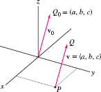
- The position vector of a point \(Q_0\) is the vector \(\textbf{v}_0 = \overrightarrow{OQ}_{\!0}\) based at the origin (Figure 12.29).
- A vector \(\textbf{v} = \overrightarrow{PQ}\) with components \(\langle a,b,c\rangle\) is equivalent to the vector \(\textbf{v}_0= \overrightarrow{OQ}_{\!0}\) based at the origin with \(Q_0 = ( a,b,c)\) (Figure 12.29).
- The components of \(\textbf{v}=\overrightarrow{PQ}\), where \(P=(a_1,b_1,c_1)\) and \(Q=(a_2,b_2,c_2)\), are the differences \(a = a_2-a_1\), \(b=b_2-b_1\), \(c=c_2-c_1\); that is, \[ \textbf{v}=\overrightarrow{PQ} = \overrightarrow{OQ}-\overrightarrow{OP} = \langle a_2,b_2,c_2\rangle - \langle a_1,b_1,c_1\rangle \] For example, if \(P=(3,-4,-4)\) and \(Q=(2,5,-1)\), then \[ \textbf{v} = \overrightarrow{PQ} = \langle2,5,-1\rangle - \langle 3,-4,-4\rangle = \langle -1,9,3\rangle \]
- Two vectors are equivalent if and only if they have the same components.
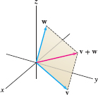
- Vector addition and scalar multiplication are defined as in the two-dimensional case. Vector addition is defined by the Parallelogram Law (Figure 12.30).
- In terms of components, if \(\textbf{v}= \langle a_1, b_1, c_1 \rangle\) and \(w= \langle a_2, b_2, c_2\rangle\), then \[ \boxed{\begin{array}{rcl} \lambda v &{}={}& \lambda\langle a_1, b_1, c_1\rangle = \langle \lambda a_1,\lambda b_1,\lambda c_1\rangle\\ \textbf{v} + w &=& \langle a_1, b_1, c_1\rangle+ \langle a_2, b_2, c_2\rangle = \langle a_1+a_2, b_1+b_2, c_1+c_2\rangle\\ \end{array}} \]
- Vector addition is commutative, is associative, and satisfies the distributive property with respect to scalar multiplication (Theorem 1 in Section 12.2).
Note
Our basepoint convention remains in force: vectors are assumed to be based at the origin unless otherwise indicated.
EXAMPLE 2 Vector Calculations
Calculate \(\parallel\textbf{v}\parallel\) and \(6v - \frac12 w\), where \(\textbf{v} = \langle 3,-1,2\rangle\) and \(w = \langle 4,6,-8\rangle\).
Solution \begin{align*} \parallel\textbf{v}\parallel &= \sqrt{3^2+(-1)^2+2^2} = \sqrt{14}\\ 6v - \frac12 w &= 6\langle 3,-1,2\rangle-\frac12\langle 4,6,-8\rangle\\ &= \langle 18,-6,12\rangle-\langle 2,3,-4\rangle\\ &= \langle 16,-9,16\rangle \end{align*}
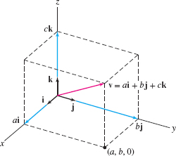
The standard basis vectors in \(\textbf{R}^3\) are \[ i = \langle 1,0,0\rangle,\qquad j=\langle 0,1,0\rangle,\qquad k = \langle 0,0,1\rangle \]
Every vector is a linear combination of the standard basis vectors (Figure 12.31): \[ \langle a,b,c\rangle = a\langle 1,0,0\rangle+b\langle 0,1,0\rangle+ c\langle 0,0,1\rangle = a i+b j +ck \]
For example, \(\langle -9,-4,17\rangle = -9i-4j+17k\).
EXAMPLE 3
Find the unit vector \(e_v\) in the direction of \(\textbf{v}=3i+2j-4k\).
Solution Since \(\parallel\textbf{v}\parallel=\sqrt{3^2+2^2+(-4)^2} = \sqrt{29}\), \[ e_v = \frac{1}{\parallel{v}\parallel}v = \frac1{\sqrt{29}}(3i+2j-4k) = \langle \frac3{\sqrt{29}},\frac2{\sqrt{29}},\frac{-4}{\sqrt{29}}\rangle \]
672
Parametric Equations of a Line
Although the basic vector concepts in two and three dimensions are essentially the same, there is an important difference in the way lines are described. A line in \(\textbf{R}^2\) is defined by a single linear equation such as \(y=mx+b\). In \(\textbf{R}^3\), a single linear equation defines a plane rather than a line. Therefore, we describe lines in \(\textbf{R}^3\) in parametric form.
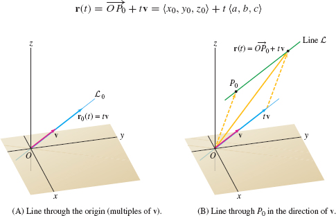
We note first that a line \(L_0\) through the origin consists of the multiples of a nonzero vector \(\textbf{v} = \langle a, b,c \rangle\), as in Figure 12.32. More precisely, set \[ r_0 = tv = \langle ta, tb, tc\rangle \qquad (-\infty \lt t \lt \infty) \]
Then the line \(L_0\) consists of the terminal points \((ta,tb,tc)\) of the vectors \(r_0\) as \(t\) varies from \(-\infty\) to \(\infty\). The coordinates \((x,y,z)\) of the points on the line are given by the parametric equations \[x= at,\quad y= bt,\quad z= ct \]
Suppose, more generally, that we would like to parametrize the line \(L\) parallel to \(\textbf{v}\) but passing through a point \(P_0 = (x_0, y_0, z_0)\) as in Figure 12.32(B). We must translate the line \(tv\) so that it passes through \(P_0\). To do this, we add the position vector \(\overrightarrow{O P_0}\) to the multiples \(tv\): \[ r(t) = \overrightarrow{OP_0}+ tv = \langle x_0, y_0, z_0\rangle + t\langle a, b,c \rangle \]
673
The terminal point of \(r(t)\) traces out \(L\) as \(t\) varies from \(-\infty\) to \(\infty\). The vector \(\textbf{v}\) is called a direction vector for \(L\), and coordinates \((x,y,z)\) of the points on the line \(L\) are given by the parametric equations \[ x =x_0+at,\quad y = y_0+bt,\quad z = z_0+ct \]
Equation of a Line (Point-Direction Form) The line \(L\) through \(P_0=(x_0,y_0,z_0)\) in the direction of \(\textbf{v}=\langle a,b,c\rangle\) is described by
Vector parametrization: \begin{equation} \boxed{r(t) = \overrightarrow{OP_0}+tv= \langle x_0, y_0, z_0 \rangle + t\langle a, b, c \rangle}\tag{5} \end{equation}
Parametric equations: \begin{equation} \boxed{x=x_0+at,\quad y=y_0+bt,\quad z=z_0+ct}\label{14.vec3.parametriclineeq}\tag{6} \end{equation}
The parameter \(t\) varies for \(-\infty \lt t \lt \infty\).
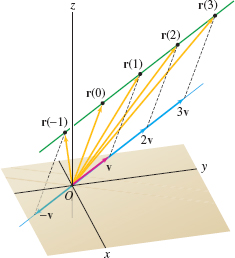
Parametric equations specify the \(x\), \(y\), and \(z\) coordinates of a point on the line as a function of the parameter \(t\). These are familiar from our discussion of parametric curves in the plane in Section 11.1. What is new here is the notion of a vector parametrization, the idea that \(r(t)\) describes a vector whose terminal point traces out a line as \(t\) varies from \(-\infty\) to \(\infty\) (Figure 12.33).
EXAMPLE 4
Find a vector parametrization and parametric equations for the line through \(P_0 = (3,-1,4)\) with direction vector \(\textbf{v}=\langle 2,1,7\rangle\).
Solution By Eq. (5), the following is a vector parametrization: \[ r(t) = {\underbrace{\langle 3,-1,4\rangle}_{\textrm{Coordinates of \(P_0\)}}} + {\,\,\,\,}t\underbrace{\langle 2,1,7\rangle}_{\textrm{ Direction vector}} = \langle 3+2t,-1+t,4+7t\rangle \]
The corresponding parametric equations are \(x=3+2t, y=-1+t, z=4+7t\).
The parametrization of a line \(L\) is not unique. We are free to choose any point \(P_0\) on \(L\) and we may replace the direction vector \(\textbf{v}\) by any nonzero scalar multiple \(\lambda v\). However, two lines in \(\textbf{R}^3\) coincide if they are parallel and pass through a common point, so we can always check whether two parametrizations describe the same line.
EXAMPLE 5 Different Parametrizations of the Same Line
Show that \[ r_1(t)=\langle 1,1,0\rangle + t\langle -2,1,3\rangle\quad\textrm{and}\quad r_2(t)=\langle -3,3,6 \rangle + t\langle 4,-2,-6\rangle \]
parametrize the same line.
Solution The line \(r_1\) has direction vector \(\textbf{v} = \langle -2,1,3\rangle\), whereas \(r_2\) has direction vector \(w = \langle 4,-2,-6\rangle\). These vectors are parallel because \(w = -2v\). Therefore, the lines described by \(r_1\) and \(r_2\) are parallel. We must check that they have a point in common. Choose any point on \(r_1\), say \(P=(1,1,0)\) [corresponding to \(t=0\)]. This point lies on \(r_2\) if there is a value of \(t\) such that \begin{equation} \langle 1,1,0\rangle = \langle -3,3,6 \rangle + t\langle 4,-2,-6\rangle\tag{7} \end{equation}
674
This yields three equations \[ 1 = -3+4t,\qquad 1 = 3-2t,\qquad 0 = 6-6t \]
All three are satisfied with \(t = 1\). Therefore \(P\) also lies on \(r_2\). We conclude that \(r_1\) and \(r_2\) parametrize the same line. If Eq. (7) had no solution, we would conclude that \(r_1\) and \(r_2\) are parallel but do not coincide.
EXAMPLE 6 Intersection of Two Lines
Determine whether the following two lines intersect: \begin{align*} r_1(t) &= \langle 1,0,1\rangle+t\langle 3,3,5\rangle\\ r_2(t) &= \langle 3,6,1\rangle+t\langle 4,-2,7\rangle \end{align*}
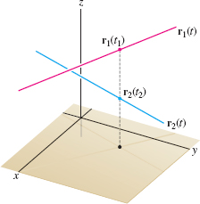
Solution The two lines intersect if there exist parameter values \(t_1\) and \(t_2\) such that \(r_1(t_1)= r_2(t_2)\)—that is, if \begin{equation} \langle 1,0,1\rangle+t_1\langle 3,3,5\rangle=\langle 3,6,1\rangle+t_2\langle 4,-2,7\rangle\tag{8} \end{equation}
This is equivalent to three equations for the components: \begin{equation} x = 1+3t_1 = 3+4t_2,\qquad y = 3t_1 = 6-2t_2,\qquad z = 1+5t_1 = 1+7t_2\tag{9} \end{equation}
Let's solve the first two equations for \(t_1\) and \(t_2\). Subtracting the second equation from the first, we get \(1 = 6t_2-3\) or \(t_2 = \frac23\). Using this value in the second equation, we get \(t_1=2-\frac23t_2=\frac{14}9\). The values \(t_1=\frac{14}9\) and \(t_2 = \frac23\) satisfy the first two equations, and thus \(r_1(t_1)\) and \(r_2(t_2)\) have the same \(x\)- and \(y\)-coordinates (Figure 12.34). However, they do not have the same \(z\)-coordinates because \(t_1\) and \(t_2\) do not satisfy the third equation in (9): \[ 1+5\left( \frac{14}9\right)\ne 1+7\left( \frac23\right) \]
Therefore, Eq. (8) has no solution and the lines do not intersect.
CAUTION
We cannot assume in Eq. (8) that the parameter values \(t_1\) and \(t_2\) are equal. The point of intersection may correspond to different parameter values on the two lines.
We can describe the line \(L\) passing through two points \(P=(a_1,b_1,c_1)\) and \(Q=(a_2,b_2,c_2)\) by the vector parametrization (Figure 12.35): \[ r(t) = (1-t)\,\overrightarrow{OP}+t\,\overrightarrow{OQ} \]
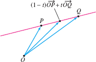
Why does \(r\) pass through \(P\) and \(Q\)? Because \(r(0) = \overrightarrow{OP}\) and \(r(1)=\overrightarrow{OQ}\). Thus \(r(t)\) traces the segment \(\overline{PQ}\) joining \(P\) and \(Q\) as \(t\) varies from \(0\) to \(1\). Explicitly, \[ r(t) = (1-t)\langle a_1,b_1,c_1\rangle+t\langle a_2,b_2,c_2\rangle \]
The parametric equations are \[ x=a_1+(a_2-a_1)t,\qquad y=b_1+(b_2-b_1)t,\qquad z=c_1+(c_2-c_1)t \]
The midpoint of \(\overline{PQ}\) corresponds to \(t=\frac12\): \[ \textrm{Midpoint of \(\overline{PQ}\)} = \left(\frac{a_1+a_2}2, \frac{b_1+b_2}2, \frac{c_1+c_2}2 \right) \]
675
Line through Two Points The line through \(P=(a_1,b_1,c_1)\) and \(Q=(a_2,b_2,c_2)\) is described by
Vector parametrization: \begin{equation} \boxed{r(t) = (1-t)\overrightarrow{O P}+t\overrightarrow{O Q} = (1-t)\langle a_1,b_1,c_1\rangle+t\langle a_2,b_2,c_2\rangle}\tag{10} \end{equation}
Parametric equations: \begin{equation} \boxed{x=a_1+(a_2-a_1)t,\quad y=b_1+(b_2-b_1)t, \quad z=c_1+(c_2-c_1)t} \end{equation}
for \(-\infty \lt t \lt \infty\). This parametrization traces the segment \(\overline{PQ}\) from \(P\) to \(Q\) as \(t\) varies from \(0\) to \(1\).
EXAMPLE 7
Parametrize the segment \(\overline{PQ}\) where \(P = (1,0,4)\) and \(Q = (3,2,1)\). Find the midpoint of the segment.
Solution The line through \(P = (1,0,4)\) and \(Q = (3,2,1)\) has the parametrization \[ r(t)= (1-t)\langle 1,0,4\rangle + t\langle 3,2,1\rangle = \langle 1+2t, 2t, 4-3t\rangle \]
The segment \(\overline{PQ}\) is traced for \(0\le t\le 1\). The midpoint of \(\overline{PQ}\) is the terminal point of the vector \[ r\left(\dfrac12\right) = \frac12\langle 1,0,4\rangle + \frac12\langle 3,2,1\rangle = \langle 2,1,\dfrac52\rangle \]
In other words, the midpoint is \(\big(2,1,\frac52\big)\).
12.3.1 Summary
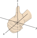
- The axes in \(\textbf{R}^3\) are labeled so that they satisfy the \emph{right-hand rule}: When the fingers of your right hand curl from the positive \(x\)-axis toward the positive \(y\)-axis, your thumb points in the positive \(z\)-direction (Figure 12.36).
Sphere of radius \(R\) and center \((a,b,c)\) \((x-a)^2+(y-b)^2+(z-c)^2=R^2 \) Cylinder of radius \(R\) with vertical axis through \((a,b,0)\) \((x-a)^2+(y-b)^2=R^2\) - The notation and terminology for vectors in the plane carry over to vectors in \(\textbf{R}^3\).
- The length (or magnitude) of \(\textbf{v}=\overrightarrow{PQ}\), where \(P=(a_1,b_1,c_1)\) and \(Q=(a_2,b_2,c_2)\), is \[ \parallel{v}\parallel = \parallel{\overrightarrow{PQ}}\parallel = \sqrt{(a_2-a_1)^2+(b_2-b_1)^2+(c_2-c_1)^2} \]
- Equations for the line through \(P_0=(x_0,y_0,z_0)\) with direction vector \(\textbf{v}=\langle a,b,c\rangle\): \begin{align*} &\textit{Vector parametrization:}&\quad &r(t) = \overrightarrow{OP}_0+tv = \langle x_0,y_0,z_0\rangle + t\langle a,b,c\rangle \\ &\textit{Parametric equations:}&\quad &x= x_0+at,\quad y = y_0+bt,\quad z = z_0+ct \end{align*}
- Equation of the line through \(P=(a_1,b_1,c_1)\) and \(Q=(a_2,b_2,c_2)\): \begin{align*} &\textit{Vector parametrization:}&\quad& r(t) = (1-t)\langle a_1,b_1,c_1\rangle+t\langle a_2,b_2,c_2\rangle\\ &\textit{Parametric equations:}&\quad &x=a_1+(a_2-a_1)t,\quad y=b_1+(b_2-b_1)t,\\ &&\quad& z=c_1+(c_2-c_1)t \end{align*}
676
The segment \(\overline{PQ}\) is parametrized by \(r(t)\) for \(0\le t\le 1\). The midpoint of \(\overline{PQ}\) is the terminal point of \(r\big(\frac12\big)\), namely \(\big(\frac12(a_1+a_2),\frac12(b_1+b_2),\frac12(c_1+c_2) \big)\).