1.5 Inverse Functions
Many important functions, such as logarithms and the arcsine, are defined as inverse functions. In this section, we review inverse functions and their graphs, and we discuss the inverse trigonometric functions.
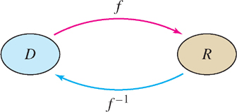
The inverse of \(f(x)\), denoted \(f^{-1}(x)\), is the function that reverses the effect of \(f(x)\) (Figure 1.58). For example, the inverse of \(f(x) = x^{3}\) is the cube root function \(f^{-1}(x) = x^{\frac{1}{3}}\).
34
Given a table of function values for \(f(x)\), we obtain a table for \(f^{-1}(x)\) by interchanging the \(x\) and \(y\) columns:
\[ \begin{array}{c} \hline \text{Function}\\ \hline \begin{array}{cc} x&y=x^3\\ \hline -2&-8\\ -1&-1\\ \phantom{-}0&\phantom{-}0\\ \phantom{-}1&\phantom{-}1\\ \phantom{-}2&\phantom{-}8\\ \phantom{-}3&\phantom{-}27 \end{array}\\ \hline \end{array} \stackrel{\text{(Interchange columns)}}{\Longrightarrow} \begin{array}{c} \hline \text{Inverse}\\ \hline \begin{array}{cc} x&y=x^3\\ \hline -8&-2\\ -1&-1\\ \phantom{-}0&\phantom{-}0\\ \phantom{-}1&\phantom{-}1\\ \phantom{-}8&\phantom{-}2\\ \phantom{-}27&\phantom{-}3 \end{array}\\ \hline \end{array} \]
If we apply both \(f\) and \(f^{-1}\) to a number \(x\) in either order, we get back \(x\). For instance,
\begin{eqnarray} \text{Apply \(f\) and then \(f^{-1}\):}\quad& 2&\xrightarrow{\text{(Apply \(x^3\))}} &8&\xrightarrow{\text{(Apply \(x^{\frac{1}{3}}\))}}&2\\ \text{Apply \(f^{-1}\) and then \(f\):}\quad& 8&\xrightarrow{\text{(Apply \(x^{\frac{1}{3}}\))}}& 2&\xrightarrow{\text{(Apply \(x^3\))}} &8\\ \end{eqnarray}
This property is used in the formal definition of the inverse function.
DEFINITION Inverse
![]() REMINDER The “domain” is the set of numbers \(x\) such that \(f (x)\) is defined (the set of allowable inputs), and the “range” is the set of all values \(f (x)\) (the set of outputs).
REMINDER The “domain” is the set of numbers \(x\) such that \(f (x)\) is defined (the set of allowable inputs), and the “range” is the set of all values \(f (x)\) (the set of outputs).
Let \(f(x)\) have domain \(D\) and range \(R\). If there is a function \(g(x)\) with domain \(R\) such that
\[ g(f(x))=x\quad\text{for }x\in D \qquad\text{and}\qquad f(g(x))=x\quad\text{for }x\in R \]
then \(f(x)\) is said to be invertible. The function \(g(x)\) is called the inverse function and is denoted \(f^{-1}(x)\).
EXAMPLE 1
Show that \(f(x) = 2x - 18\) is invertible. What are the domain and range of \(f^{-1}(x)\)?
Solution We show that \(f(x)\) is invertible by computing the inverse function in two steps.
Step 1. Solve the equation \(y = f(x)\) for \(x\) in terms of \(y\)
\begin{align*} y&=2x-18\\[5pt] y+18&=2x\\[5pt] x&=\frac{1}{2}y+9 \end{align*}
This gives us the inverse as a function of the variable \(y\): \(f^{-1}(y)=\frac{1}{2}y+9\)
Step 2. Interchange variables.
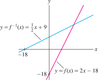
We usually prefer to write the inverse as a function of \(x\), so we interchange the roles of \(x\) and \(y\) (Figure 1.59):
\[ f^{-1}(x)=\frac{1}{2}x+9 \]
To check our calculation, let’s verify that \(f^{-1}(f(x)) = x\) and \(f (f^{-1} (x)) = x\):
\begin{align*} f^{-1}(f(x))&=f^{-1}(2x-18) = \frac{1}{2}(2x-18)+9 =(x-9)+9=x\\[5pt] f(f^{-1}(x))&=f\left(\frac{1}{2}x+9\right)=2\left(\frac{1}{2}y+9\right)-18= (x+18)-18=x \end{align*}
Because \(f^{-1}\) is a linear function, its domain and range are \(\mathbb{R}\).
35
The inverse function, if it exists, is unique. However, some functions do not have an inverse. Consider \(f(x) = x^{2}\). When we interchange the columns in a table of values (which should give us a table of values for \(f^{-1}\)), the resulting table does not define a function:
\[\left. \begin{array}{c} \hline \text{Function}\\ \hline \begin{array}{cc} x&y=x^2\\ \hline -2&4\\ -1&{\bf 1}\\ \phantom{-}0&0\\ \phantom{-}1&{\bf 1}\\ \phantom{-}2&4 \end{array}\\ \hline \end{array} \stackrel{\text{(Interchange columns)}}{\Longrightarrow} \begin{array}{c} \hline \text{Inverse}\\ \hline \begin{array}{cc} x&y=x^3\\ \hline 4&-2\\ {\bf 1}&-1\\ 0&\phantom{-}0\\ {\bf 1}&\phantom{-}1\\ 4&\phantom{-}2 \end{array}\\ \hline \end{array} \right\} \begin{array}{l} \text{\(f^{-1}\) has two}\\ \text{values: 1 and -1} \end{array} \]
The problem is that every positive number occurs twice as an output of \(f(x) = x^{2}\). For example, 1 occurs twice as an output in the first table and therefore occurs twice as an input in the second table. So the second table gives us two possible values for \(f^{-1}(1)\), namely \(f^{-1}(1) = 1\) and \(f^{-1}(1) = -1\). Neither value satisfies the inverse property. For instance, if we set \(f^{-1}(1) = 1\), then \(f^{-1} (f (-1)) = f^{-1}(1) = 1\), but an inverse would have to satisfy \(f^{-1} (f(-1)) = -1\).
Another standard term for one-to-one is injective.
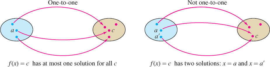
So when does a function \(f(x)\) have an inverse? The answer is: If \(f(x)\) is one-to-one, which means that \(f(x)\) takes on each value at most once (Figure 1.60). Here is the formal definition:
DEFINITION One-to-One Function
A function \(f(x)\) is one-to-one on a domain \(D\) if, for every value \(c\), the equation \(f(x) = c\) has at most one solution for \(x \in D\). Or, equivalently, if for all \(a, b \in D\),
\[ f(a)\neq f(b)\quad\text{unless}\quad a=b \]
Think of a function as a device for “labeling” members of the range by members of the domain. When \(f\) is one-to-one, this labeling is unique and \(f^{-1}\) maps each number in the range back to its label.
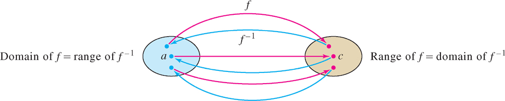
When \(f(x)\) is one-to-one on its domain \(D\), the inverse function \(f^{-1}(x)\) exists and its domain is equal to the range \(R\) of \(f\) (Figure 1.61). Indeed, for every \(c \in R\), there is precisely one element \(a \in D\) such that \(f(a) = c\) and we may define \(f^{-1}(c) = a\). With this definition, \(f(f^{-1}(c)) = f(a) = c\) and \(f^{-1}(f(a)) = f^{-1}(c) = a\). This proves the following theorem.
36
THEOREM 1 Existence of Inverses
The inverse function \(f^{-1}(x)\) exists if and only if \(f(x)\) is one-to-one on its domain \(D\). Furthermore,
- \(\text{Domain of }f=\text{Range of }f^{-1}\).
- \(\text{Range of }f=\text{Domain of }f^{-1}\).
Often, it is impossible to find a formula for the inverse because we cannot solve for \(x\) explicitly in the equation \(y = f(x)\). For example, the function \(f(x) = x + e^{x}\) has an inverse, but we must make do without an explicit formula for it.
EXAMPLE 2
Show that \(f(x)=\frac{3x+2}{5x-1}\) is invertible. Determine the domain and range of \(f\) and \(f^{-1}\).
Solution The domain of \(f(x)\) is \(D=\{x:x\neq\frac{1}{5}\}\) (Figure 1.62). Assume that \(x \in D\), and let’s solve \(y = f(x)\) for \(x\) in terms of \(y\):
\begin{align*} y&=\frac{3x+2}{5x-1}\\[5pt] y(5x-1)&=3x+2\\[5pt] 5xy-y&=3x+2\\[5pt] 5xy-3x&=y+2&&\text{(gather terms involving \(x\))}\\[5pt] x(5y-3)&=y+2&&\text{(factor out \(x\) in order to solve for \(x\))}\tag{1}\\[5pt] x&=\frac{y+2}{5y-3}&&\text{(divide by \(5y-3\))}\tag{2} \end{align*}
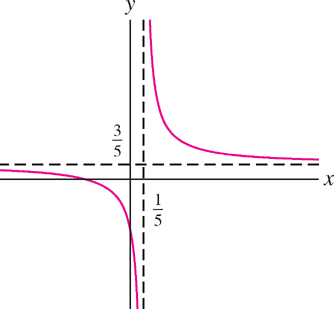
The last step is valid if \(5y -3 \neq 0\) —that is, if \(y\neq\frac{3}{5}\). But note that \(y=\frac{3}{5}\) is not in the range of \(f(x)\). For if it were, Eq. (1) would yield the false equation \(0=\frac{3}{5}+2\). Now Eq. (2) shows that for all \(y\neq\frac{3}{5}\), there is a unique value \(x\) such that \(f(x) = y\). Therefore, \(f(x)\) is one-to-one on its domain. By Theorem 1, \(f(x)\) is invertible. The range of \(f(x)\) is \(R=\{x:x\neq\frac{3}{5}\}\) and
\[ f^{-1}(x)= \frac{x+2}{5x-3} \]
The inverse function has domain \(R\) and range \(D\).
We can tell whether \(f(x)\) is one-to-one from its graph. The horizontal line \(y = c\) intersects the graph of \(f(x)\) at points \((a, f(a))\), where \(f(a) = c\) (Figure 1.63). There is at most one such point if \(f(x) = c\) has at most one solution. This gives us the
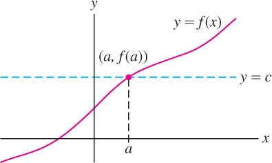
Horizontal Line Test A function \(f(x)\) is one-to-one if and only if every horizontal line intersects the graph of \(f(x)\) in at most one point.
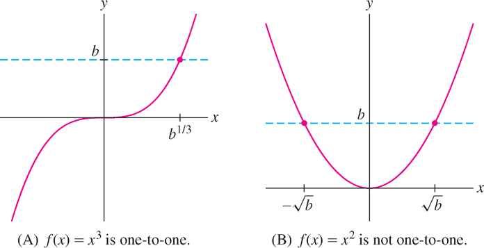
In Figure 1.64, we see that \(f(x) = x^{3}\) passes the Horizontal Line Test and therefore is one-to-one, whereas \(f(x) = x^{2}\) fails the test and is not one-to-one.
EXAMPLE 3 Increasing Functions Are One-to-One
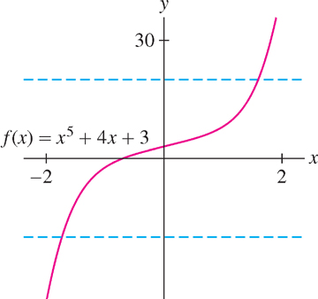
Show that increasing functions are one-to-one. Then show that \(f(x) = x^{5} + 4x + 3\) is one-to-one.
Solution An increasing function satisfies \(f(a) < f(b)\) if \(a < b\). Therefore \(f\) cannot take on any value more than once, and thus \(f\) is one-to-one. Note similarly that decreasing functions are one-to-one.
37
Now observe that
- If \(n\) odd and \(c > 0\), then \(cx^{n}\) is increasing.
- A sum of increasing functions is increasing.
Thus \(x^{5}, 4x\), and hence the sum \(x^{5} + 4x\) is increasing. It follows that \(f(x) = x^{5} + 4x + 3\) is increasing and therefore one-to-one (Figure 1.65).
We can make a function one-to-one by restricting its domain suitably.
EXAMPLE 4 Restricting the Domain
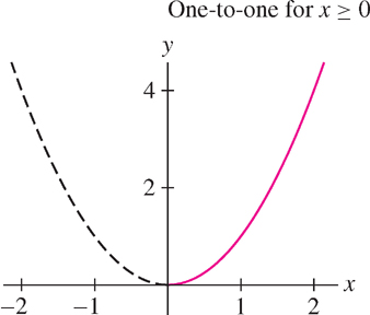
Find a domain on which \(f(x) = x^{2}\) is one-to-one and determine its inverse on this domain.
Solution The function \(f(x) = x^{2}\) is one-to-one on the domain \(D = \{x : x \geq 0\}\), for if \(a^{2} = b^{2}\) where \(a\) and \(b\) are both nonnegative, then \(a = b\) (Figure 1.66). The inverse of \(f(x)\) on \(D\) is the positive square root \(f^{-1}(x)=\sqrt{x}\). Alternatively, we may restrict \(f(x)\) to the domain \(\{x : x \leq 0\}\), on which the inverse function is \(f^{-1}(x)=-\sqrt{x}\).
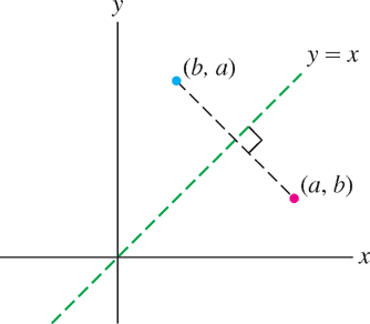
Next we describe the graph of the inverse function. The reflection of a point \((a, b)\) through the line \(y = x\) is, by definition, the point \((b, a)\) (Figure 1.67). Note that if the \(x\)- and \(y\)-axes are drawn to the same scale, then \((a, b)\) and \((b, a)\) are equidistant from the line \(y = x\) and the segment joining them is perpendicular to \(y = x\).
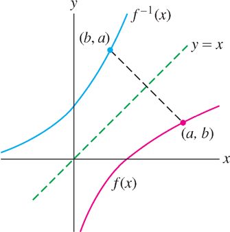
The graph of \(f^{-1}\) is the reflection of the graph of \(f\) through \(y = x\) (Figure 1.68). To check this, note that \((a, b)\) lies on the graph of \(f\) if \(f(a) = b\). But \(f(a) = b\) if and only if \(f^{-1}(b) = a\), and in this case, \((b, a)\) lies on the graph of \(f^{-1}\).
38
EXAMPLE 5 Sketching the Graph of the Inverse
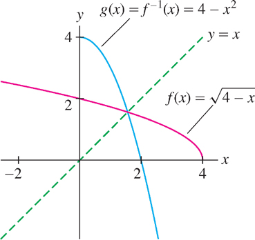
Sketch the graph of the inverse of \(f(x)=\sqrt{4-x}\).
Solution Let \(g(x) = f^{-1}(x)\). Observe that \(f(x)\) has domain \(\{x : x \leq 4\}\) and range \(\{x : x \geq 0\}\). We do not need a formula for \(g(x)\) to draw its graph. We simply reflect the graph of \(f\) through the line \(y = x\) as in Figure 1.69. If desired, however, we can easily solve \(y=\sqrt{4-x}\) to obtain \(x = 4 - y^{2}\) and thus \(g(x) = 4 - x^{2}\) with domain \(\{x : x \geq 0\}\).
1.5.1 Inverse Trigonometric Functions
Do not confuse the inverse \(\sin^{-1} x\) with the reciprocal
\[ (\sin x)^{-1}=\frac{1}{\sin x}=\csc x \]
The inverse functions \(\sin^{-1} x, \cos^{-1} x,\ldots\) are often denoted \(\text{arcsin}\,x, \text{arccos}\,x,\) etc.
We have seen that the inverse function \(f^{-1}(x)\) exists if and only if \(f(x)\) is one-to-one on its domain. Because the trigonometric functions are not one-to-one, we must restrict their domains to define their inverses.
First consider the sine function. Figure 1.70 shows that \(f(\theta ) = \sin \theta \) is one-to-one on \([-\frac{\pi}{2},\frac{\pi}{2}]\). With this interval as domain, the inverse is called the arcsine function and is denoted \(\theta=\sin^{-1} x\) or \(\theta=\text{arcsin}\,x\). By definition,
\[ \boxed{\theta=\sin^{-1}x\text{ is the unique angle in } \left[-\dfrac{\pi}{2},\dfrac{\pi}{2}\right] \text{ such that } \sin\theta=x} \]
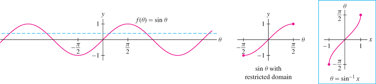
The range of \(\sin x\) is \([-1, 1]\), so \(\sin^{-1}x\) has domain \([-1, 1]\). A table of values for the arcsine (Table 1.7) is obtained by reversing the columns in a table of values for \(\sin x\).
Summary of inverse relation between the sine and arcsine functions:
\begin{align*} \sin(\sin^{-1}x)&=x&\hspace{-10pt}& \text{for }-1\leq x\leq1\\[5pt] \sin^{-1}(\sin\theta)&=\theta&\hspace{-10pt}& \text{for }-\frac{\pi}{2}\leq\theta\leq\frac{\pi}{2} \end{align*}
| \[ \begin{array}{c} \hline \text{Table 1.7}\\[5pt] \hline \begin{array}{lccccccccc} x&-1&-\tfrac{\sqrt{3}}{2}&-\tfrac{\sqrt2}{2} &-\tfrac{1}{2}&0&\tfrac{1}{2}&\tfrac{\sqrt2}{2}&\tfrac{\sqrt3}{2}&1\\ \theta=\sin^{-1}x&-\tfrac{\pi}{2}&-\tfrac{\pi}{3}&-\tfrac{\pi}{4}&-\tfrac{\pi}{6}&0&\tfrac{\pi}{6}&\tfrac{\pi}{4}&\tfrac{\pi}{3}&\tfrac{\pi}{2} \end{array}\\ \hline \end{array} \] |
EXAMPLE 6
(a) Show that \(\sin^{-1}(\sin(\frac{\pi}{4}))=\frac{\pi}{4}\).
(b) Explain why \(\sin^{-1}(\sin(\frac{5\pi}{4}))\neq\frac{5\pi}{4}\).
Solution The equation \(\sin^{-1} (\sin \theta ) = \theta \) is valid only if \(\theta \) lies in \([-\frac{\pi}{2},\frac{\pi}{2}]\).
(a) Because \(\frac{\pi}{4}\) lies in the required interval, \([-\frac{\pi}{2},\frac{\pi}{2}]\).
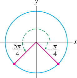
(b) Let \(\theta=\sin^{-1}(\sin(\frac{5\pi}{4}))\). By definition, \(\theta \) is the angle in \([-\frac{\pi}{2},\frac{\pi}{2}]\) such that \(\sin\theta=\sin(\frac{5\pi}{4})\). By the identity \(\sin\theta=\sin(\pi-\theta)\) (Figure 1.71),
39
\[ \sin(\frac{5\pi}{4})=\sin(\pi-\frac{5\pi}{4})=\sin(-\frac{\pi}{4}) \] The angle \(-\frac{\pi}{2}\) lies in the required interval, so \(\theta = \sin^{-1}(\sin(\frac{5\pi}{4}))=-\frac{\pi}{4}\).
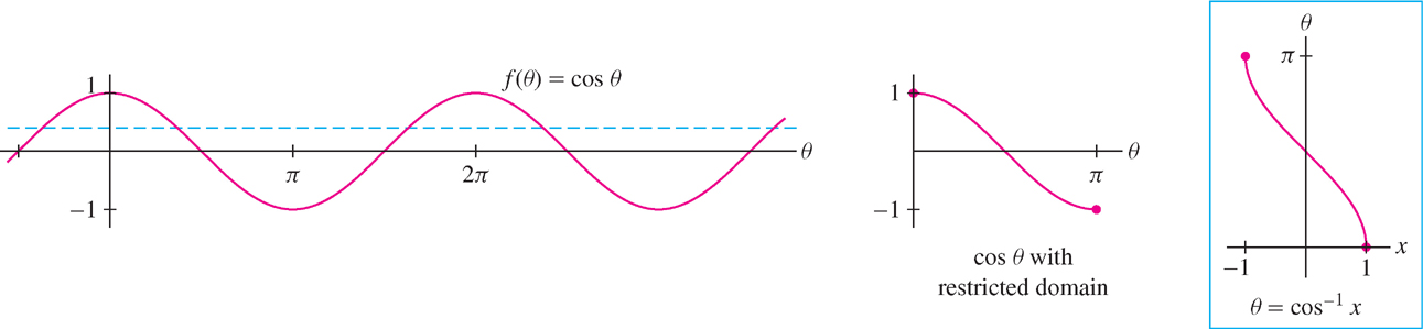
Summary of inverse relation between the cosine and arccosine:
\begin{align*} \cos(\cos^{-1}x)&=x&\hspace{-10pt}& \text{for }-1\leq x\leq1\\[5pt] \cos^{-1}(\cos\theta)&=\theta&\hspace{-10pt}& \text{for }0\leq\theta\leq\pi \end{align*}
The cosine function is one-to-one on \([0, \pi ]\) rather than \([-\frac{\pi}{2},\frac{\pi}{2}]\) (Figure 1.72). With this domain, the inverse is called the arccosine function and is denoted \(\theta = \cos^{-1} x\) or \(\theta = \text{arccos}\,x\). It has domain \([-1, 1]\). By definition,
\[ \boxed{\theta=\cos^{-1}x\text{ is the unique angle in } [0,\pi] \text{ such that } \cos\theta=x} \]
THIS PARA. IS JUST FOR SPACING. REMOVED AT PUBLISH BY STYLING.
When we study the calculus of inverse trigonometric functions in Section 3.8, we will need to simplify composite expressions such as \(\cos(\sin^{-1} x)\) and \(\tan(\sin^{-1} x)\). This can be done in two ways: by referring to the appropriate right triangle or by using trigonometric identities.
EXAMPLE 7
Simplify \(\cos(\sin^{-1} x)\) and \(\tan(\sin^{-1} x)\).
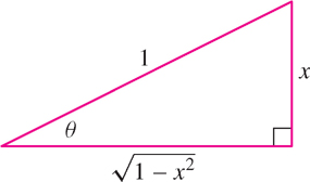
Solution This problem asks for the values of \(\cos\theta \) and \(tan \theta \) at the angle \(\theta = sin^{-1} x\). Consider a right triangle with hypotenuse of length 1 and angle \(\theta \) such that \(\sin \theta = x\), as in Figure 1.73. By the Pythagorean Theorem, the adjacent side has length \(\sqrt{1-x^2}\). Now we can read off the values from Figure 1.73:
\begin{align*} \cos(\sin^{-1} x )&=\cos\theta= \frac{\text{adjacent}}{\text{hypotenuse}}=\sqrt{1-x^2}\\ \tan(\sin^{-1} x )&=\tan\theta= \frac{\text{opposite}}{\text{adjacent}}=\frac{x}{\sqrt{1-x^2}} \end{align*}
Alternatively, we may argue using trigonometric identities. Because \(\sin \theta = x\),
\[ \cos(\sin^{-1}x)=\cos\theta = \sqrt{1-\sin^2\theta} = \sqrt{1-x^2} \]
We are justified in taking the positive square root because \(\theta = \sin^{-1} x\) lies in \([-\frac{\pi}{2},\frac{\pi}{2}]\) and \(\cos \theta \) is positive in this interval.
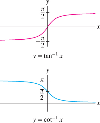
We now address the remaining trigonometric functions. The function \(f(\theta ) = \tan\theta \) is one-to-one on \((-\frac{\pi}{2},\frac{\pi}{2})\), and \(f(\theta ) = \cot \theta \) is one-to-one on \((0, \pi )\) [see Figure 1.48 in Section 1.4]. We define their inverses by restricting them to these domains:
\begin{gather*} \boxed{\theta=\tan^{-1}x\text{ is the unique angle in } \left(-\dfrac{\pi}{2},\dfrac{\pi}{2}\right) \text{ such that } \tan\theta=x}\\ \boxed{\theta=\cot^{-1}x\text{ is the unique angle in } (0,\pi) \text{ such that } \cot\theta=x} \end{gather*}
40
The range of both \(\tan \theta \) and \(\cot \theta \) is the set of all real numbers \(\mathbb{R}\). Therefore, \(\theta = \tan^{-1} x\) and \(\theta= \cot^{-1} x\) have domain \(\mathbb{R}\) (Figure 1.74).
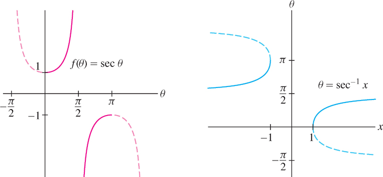
The function \(f(\theta ) = \sec \theta \) is not defined at \(\theta=\frac{\pi}{2}\), but we see in Figure 1.75 that it is one-to-one on both \([0,\frac{\pi}{2})\) and \((\frac{\pi}{2},\pi]\). Similarly, \(f(\theta ) = \csc \theta \) is not defined at \(\theta = 0\), but it is one-to-one on \([-\frac{\pi}{2},0)\) and \((0,\frac{\pi}{2}]\). We define the inverse functions as follows:
\begin{gather*} \boxed{\theta=\sec^{-1}x\text{ is the unique angle in } \left[0,\dfrac{\pi}{2}\right)\cup\left(\dfrac{\pi}{2},\pi\right] \text{ such that } \sec\theta=x}\\ \boxed{\theta=\csc^{-1}x\text{ is the unique angle in } \left[-\dfrac{\pi}{2},0\right)\cup\left(0,\dfrac{\pi}{2}\right] \text{ such that } \csc\theta=x}\\ \end{gather*}
Figure 1.75 shows that the range of \(f(\theta ) = \sec \theta \) is the set of real numbers \(x\) such that \(|x| \geq 1\). The same is true of \(f(\theta ) = \csc \theta \). It follows that both \(\theta = \sec^{-1} x\) and \(\theta = csc^{-1} x\) have domain \(\{x: |x| \geq 1\}\).
1.5.2 Section 1.5 Summary
- A function \(f(x)\) is one-to-one on a domain \(D\) if for every value \(c\), the equation \(f(x) = c\) has at most one solution for \(x \in D\), or, equivalently, if for all \(a, b \in D\), \(f(a) \neq f(b)\) unless \(a = b\).
- Let \(f(x)\) have domain \(D\) and range \(R\). The inverse \(f^{-1}(x)\) (if it exists) is the unique function with domain \(R\) and range \(D\) satisfying \(f(f^{-1}(x)) = x\) and \(f^{-1}(f(x)) = x\).
- The inverse of \(f(x)\) exists if and only if \(f(x)\) is one-to-one on its domain.
- To find the inverse function, solve \(y = f(x)\) for \(x\) in terms of \(y\) to obtain \(x = g(y)\). The inverse is the function \(g(x)\).
- Horizontal Line Test: \(f(x)\) is one-to-one if and only if every horizontal line intersects the graph of \(f(x)\) in at most one point.
- The graph of \(f^{-1}(x)\) is obtained by reflecting the graph of \(f(x)\) through the line \(y = x\).
- The arcsine and arccosine are defined for \(-1 \leq x \leq 1\):
\(\theta=\sin^{-1}x\) is the unique angle in \([-\frac{\pi}{2},\frac{\pi}{2}]\) such that \(\sin\theta=x\).
\(\theta=\cos^{-1}x\) is the unique angle in \([0,\pi]\) such that \(\cos\theta=x\).
41
- \(\tan^{-1} x\) and \(\cot^{-1} x\) are defined for all \(x\):
\(\theta=\tan^{-1}x\) is the unique angle in \((-\frac{\pi}{2},\frac{\pi}{2})\) such that \(\tan\theta=x\).
\(\theta=\cot^{-1}x\) is the unique angle in \((0,\pi)\) such that \(\cot\theta=x\).
- \(\sec^{-1} x\) and \(\csc^{-1} x\) are defined for \(|x| \geq 1\):
\(\theta=\sec^{-1}x\) is the unique angle in \([0,\frac{\pi}{2})\cup(\frac{\pi}{2},\pi]\) such that \(\sec\theta=x\)
\(\theta=\csc^{-1}x\) is the unique angle in \([-\frac{\pi}{2},0)\cup(0,\dfrac{\pi}{2}]\) such that \(\csc\theta=x\)