1.7 Technology: Calculators and Computers
Computer technology has vastly extended our ability to calculate and visualize mathematical relationships. In applied settings, computers are indispensable for solving complex systems of equations and analyzing data, as in weather prediction and medical imaging. Mathematicians use computers to study complex structures such as the Mandelbrot Set (Figure 1.81 and Figure 1.82). We take advantage of this technology to explore the ideas of calculus visually and numerically.
52


When we plot a function with a graphing calculator or computer algebra system, the graph is contained within a viewing rectangle, the region determined by the range of \(x\)- and \(y\)-values in the plot. We write \([a, b] \times [c, d]\) to denote the rectangle where \(a \leq x \leq b\) and \(c \leq y \leq d\).
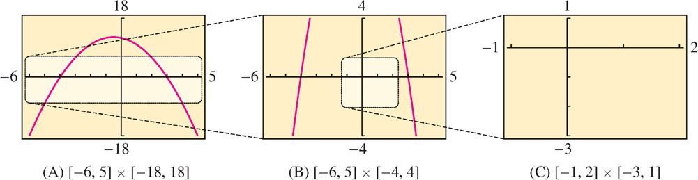
The appearance of the graph depends heavily on the choice of viewing rectangle. Different choices may convey very different impressions which are sometimes misleading. Compare the three viewing rectangles for the graph of \(f(x) = 12 - x - x^{2}\) in Figure 1.83. Only (A) successfully displays the shape of the graph as a parabola. In (B), the graph is cut off, and no graph at all appears in (C). Keep in mind that the scales along the axes may change with the viewing rectangle. For example, the unit increment along the \(y\)-axis is larger in (B) than in (A), so the graph in (B) is steeper.
There is no single “correct” viewing rectangle. The goal is to select the viewing rectangle that displays the properties you wish to investigate. This usually requires experimentation.
EXAMPLE 1 How Many Roots and Where?
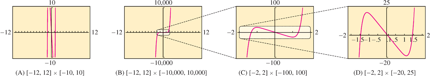
How many real roots does the function \(f(x) = x^{9} - 20x + 1\) have? Find their approximate locations.
Solution We experiment with several viewing rectangles (Figure 1.84). Our first attempt (A) displays a cut-off graph, so we try a viewing rectangle that includes a larger range of \(y\)-values. Plot (B) shows that the roots of \(f(x)\) lie somewhere in the interval \([-3, 3]\), but it does not reveal how many real roots there are. Therefore, we try the viewing rectangle in (C). Now we can see clearly that \(f(x)\) has three roots. A further zoom in (D) shows that these roots are located near \(-1.5\), \(0.1\), and \(1.5\). Further zooming would provide their locations with greater accuracy.
53
EXAMPLE 2 Does a Solution Exist?
Does \(\cos x = \tan x\) have a solution? Describe the set of all solutions.
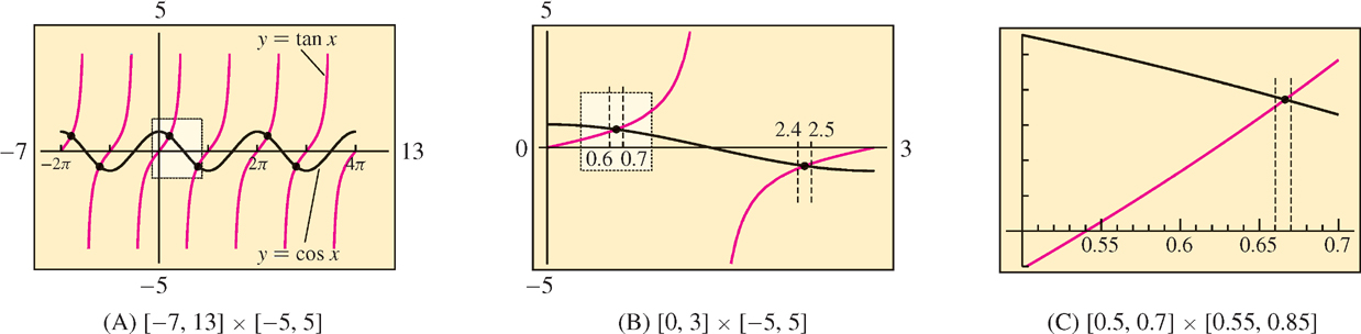
Solution The solutions of \(\cos x = \tan x\) are the \(x\)-coordinates of the points where the graphs of \(y = \cos x\) and \(y = \tan x\) intersect. Figure 1.85(A) shows that there are two solutions in the interval \([0, 2\pi]\). By zooming in on the graph as in (B), we see that the first positive root lies between \(0.6\) and \(0.7\) and the second positive root lies between \(2.4\) and \(2.5\). Further zooming shows that the first root is approximately \(0.67\) [Figure 1.85(C)]. Continuing this process, we find that the first two roots are \(x \approx 0.666\) and \(x \approx 2.475\).
Since \(\cos x\) and \(\tan x\) are periodic, the picture repeats itself with period \(2\pi\). All solutions are obtained by adding multiples of \(2\pi \) to the two solutions in \([0, 2\pi ]\):
\[ x\approx0.666+2\pi k \quad\text{and}\quad x\approx2.475+2\pi k\quad\text{(for any integer \(k\))} \]
EXAMPLE 3 Functions with Asymptotes
Plot the function \(f(x)=\frac{1-3x}{x-2}\) and describe its asymptotic behavior.
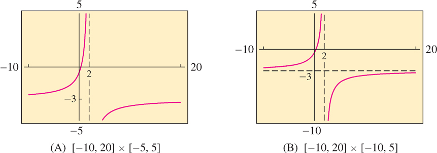
Solution First, we plot \(f(x)\) in the viewing rectangle \([-10, 20] \times [-5, 5]\) as in Figure 1.86(A). The vertical line \(x = 2\) is called a vertical asymptote. Many graphing calculators display this line, but it is not part of the graph (and it can usually be eliminated by choosing a smaller range of \(y-\)values). We see that \(f(x)\) tends to \(\infty\) as \(x\) approaches \(2\) from the left, and to \(-\infty\) as \(x\) approaches \(2\) from the right. To display the horizontal asymptotic behavior of \(f(x)\), we use the viewing rectangle \([-10, 20] \times [-10, 5]\) [Figure 1.86(B)]. Here we see that the graph approaches the horizontal line \(y = -3\), called a horizontal asymptote (which we have added as a dashed horizontal line in the figure).
Technology is indispensable but also has its limitations. When shown the computer-generated results of a complex calculation, the Nobel prize–winning physicist Eugene Wigner (1902–1995) is reported to have said: "It is nice to know that the computer understands the problem, but I would like to understand it too."
54
Calculators and computer algebra systems give us the freedom to experiment numerically. For instance, we can explore the behavior of a function by constructing a table of values. In the next example, we investigate a function related to exponential functions and compound interest (see Section 5.8).
EXAMPLE 4 Investigating the Behavior of a Function
| \(n\) | \(\left(1+\dfrac{1}{n}\right)^{n}\) |
| \(10\) | \(2.59374\) |
| \(10^{2}\) | \(2.70481\) |
| \(10^{3}\) | \(2.71692\) |
| \(10^{4}\) | \(2.71815\) |
| \(10^{5}\) | \(2.71827\) |
| \(10^{6}\) | \(2.71828\) |
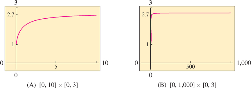
How does \(f(n) = (1 + 1/n)^{n}\) behave for large whole-number values of \(n\)? Does \(f(n)\) tend to infinity as \(n\) gets larger?
Solution First, we make a table of values of \(f(n)\) for larger and larger values of \(n\). Table 1.9 suggests that \(f(n)\) does not tend to infinity. Rather, as \(n\) grows larger, \(f(n)\) appears to get closer to some value near 2.718 (a number resembling \(e\)). This is an example of limiting behavior that we will discuss in Chapter 2. Next, replace \(n\) by the variable \(x\) and plot the function \(f(x) = (1 + 1/x)^{x}\). The graphs in Figure 1.87 confirm that \(f(x)\) approaches a limit of approximately \(2.7\). We will prove that \(f(n)\) approaches \(e\) as \(n\) tends to infinity in Section 5.8.
EXAMPLE 5 Bird Flight: Finding a Minimum Graphically
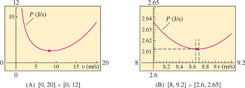
According to one model of bird flight, the power consumed by a pigeon flying at velocity \(v\) (in meters per second) is \(P(v) = 17v^{-1} + 10^{-3}v^{3}\) (in joules per second). Use a graph of \(P(v)\) to find the velocity that minimizes power consumption.
Solution The velocity that minimizes power consumption corresponds to the lowest point on the graph of \(P(v)\). We plot \(P(v)\) first in a large viewing rectangle (Figure 1.88). This figure reveals the general shape of the graph and shows that \(P(v)\) takes on a minimum value for \(v\) somewhere between \(v = 8\) and \(v = 9\). In the viewing rectangle \([8, 9.2] \times [2.6, 2.65]\), we see that the minimum occurs at approximately \(v = 8.65\text{ m/s}\).
55
Local linearity is an important concept in calculus that is based on the idea that many functions are nearly linear over small intervals. Local linearity can be illustrated effectively with a graphing calculator.
EXAMPLE 6 Illustrating Local Linearity
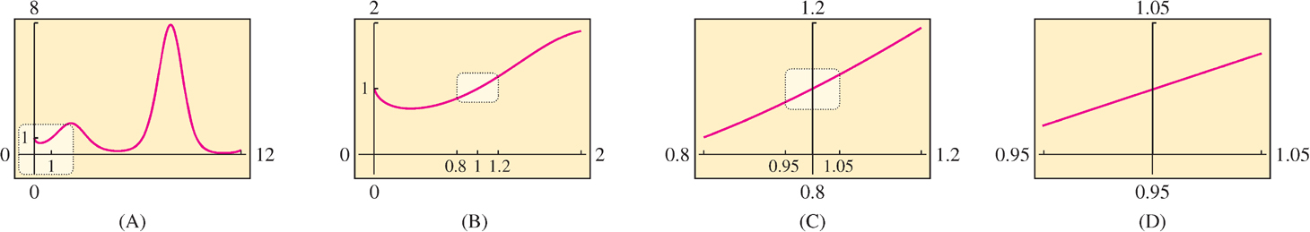
Illustrate local linearity for the function \(f(x) = x^{\sin x}\) at \(x = 1\).
Solution First, we plot \(f(x) = x^{\sin x}\) in the viewing window of Figure 1.89(A). The graph moves up and down and appears very wavy. However, as we zoom in, the graph straightens out. Figures (B)–(D) show the result of zooming in on the point \((1, f(1))\). When viewed up close, the graph looks like a straight line. This illustrates the local linearity of \(f(x)\) at \(x = 1\).
1.7.1 Section 1.7 Summary
- The appearance of a graph on a graphing calculator depends on the choice of viewing rectangle. Experiment with different viewing rectangles until you find one that displays the information you want. Keep in mind that the scales along the axes may change as you vary the viewing rectangle.
- The following are some ways in which graphing calculators and computer algebra systems can be used in calculus:
- – Visualizing the behavior of a function
- – Finding solutions graphically or numerically
- – Conducting numerical or graphical experiments
- – Illustrating theoretical ideas (such as local linearity)