2.1 Limits, Rates of Change, and Tangent Lines
Rates of change play a role whenever we study the relationship between two changing quantities. Velocity is a familiar example (the rate of change of position with respect to time), but there are many others, such as

- The infection rate of an epidemic (newly infected individuals per month)
- Inflation rate (change in consumer price index per year)
- Rate of change of atmospheric temperature with respect to altitude
Roughly speaking, if \(y\) and \(x\) are related quantities, the rate of change should tell us how much \(y\) changes in response to a unit change in \(x\). For example, if an automobile travels at a velocity of 80 km/hr, then its position changes by 80 km for each unit change in time (the unit being 1 hour). If the trip lasts only half an hour, its position changes by 40 km, and in general, the change in position is 80\(t\) km, where \(t\) is the change in time (that is, the time elapsed in hours). In other words,
Change in Position = Velocity \(\times\) Change in Time
However, this simple formula is not valid or even meaningful if the velocity is not constant. After all, if the automobile is accelerating or decelerating, which velocity would we use in the formula?
The problem of extending this formula to account for changing velocity lies at the heart of calculus. As we will learn, differential calculus uses the limit concept to define instantaneous velocity, and integral calculus enables us to compute the change in position in terms of instantaneous velocity. But these ideas are very general. They apply to all rates of change, making calculus an indispensable tool for modeling an amazing range of real-world phenomena.
In this section, we discuss velocity and other rates of change, emphasizing their graphical interpretation in terms of tangent lines. Although at this stage, we cannot define precisely what a tangent line is—this will have to wait until Chapter 3—you can think of a tangent line as a line that skims a curve at a point, as in Figure 2.1(A) and (B) but not (C).
41
2.1.1 Velocity
When we speak of velocity, we usually mean instantaneous velocity, which indicates the speed and direction of an object at a particular moment. The idea of instantaneous velocity makes intuitive sense, but care is required to define it precisely.
In linear motion, velocity may be positive or negative (indicating the direction of motion). Speed, by definition, is the absolute value of velocity and is always non-negative.
Consider an object traveling in a straight line (linear motion). The average velocity over a given time interval has a straightforward definition as the ratio\[\text{Average Velocity} = \frac{\text{change in position}}{\text{length of time interval}}\]For example, if an automobile travels 200 km in 4 hours, then its average velocity during this 4-hour period is \(\frac{200}{4}= 50 \) km/h. At any given moment the automobile may be going faster or slower than the average.
42
Question 2.1 Average Velocity Progress Check
What is the average velocity (in kilometers per hour, or km/h) of an automobile that travels 30 km in 20 minutes?
| A. |
| B. |
| C. |
We cannot define instantaneous velocity as a ratio in the same way because we would have to divide by the length of the time interval (which is zero). However, we should be able to estimate instantaneous velocity by computing average velocity over successively smaller time intervals. The guiding principle is: Average velocity over a very small time interval is very close to instantaneous velocity. To explore this idea further, we introduce some notation.
The Greek letter \(\Delta\) (Delta) is commonly used to denote the change in a function or variable. If \(s(t)\) is the position of an object (distance from the origin) at time \(t\) and \([t_0,t_1]\) is a time interval, we set \[\begin{array}{rll} \Delta s & = s(t_1) - s(t_0) & = \text{change in position}\\ \Delta t & = t_1 - t_0 & = \text{change in time (length of time interval)} \end{array}\] The change in position \(\Delta(s)\) is also called the displacement, or net change in position. For \(t_1 \neq t_0\),\[\text{Average velocity over }[t_0,t_1]=\frac{\Delta s}{\Delta t} = \frac{s(t_1) - s(t_0)}{t_1 - t_0}\]One motion we will study is the motion of an object falling to earth under the influence of gravity (assuming no air resistance). Galileo discovered that if the object is released at time \(t=0\) from a state of rest (Figure 2.2), then the distance dropped after \(t\) seconds is \(4.9t^2\) meters. This means in particular that if the object is dropped from a height \(H\) meters relative to some fixed reference frame (such as the ground), then the position or height of the object at time \(t\) is given by the formula \( s(t) = H-4.9t^2\).
EXAMPLE 1
A stone, released from a state of rest, falls to earth from a height of 50 meters above the ground (this is approximately the height of the leaning tower of Pisa, Italy). Estimate the instantaneous velocity of the stone at \(t = 0.8 s\), assuming that the stone is only affected by the gravitational pull of the earth, i.e. we assume there is no wind or air resistance.
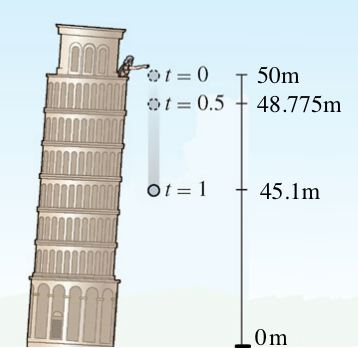
Solution Following Galileo, we use the formula \(s(t) = 50-4.9t^2\) to compute the average velocity over the five short time intervals listed in Table 2.1. Consider the first interval \([t_0,t_1]= [0.8, 0.81]\): \begin{align*} \Delta s & = s(0.81) - s(0.8) = (50 - 4.9 (0.81)^2) - (50 - 4.9 (0.8)^2) \\ &= 3.136 - 3.21489 = -0.07889 \text{ m} \\ \Delta t & = 0.81 - 0.8 = 0.01 \text{ s} \end{align*}
| Time intervals | Average velocity (m/s) |
|---|---|
| \([0.8, 0.81]\) | \(-7.889\) |
| \([0.8, 0.805]\) | \(-7.8645\) |
| \([0.8, 0.8001]\) | \(-7.8405\) |
| \([0.8, 0.80005]\) | \(-7.84024\) |
| \([0.8, 0.800001]\) | \(-7.840005\) |
The average velocity over \([0.8, 0.81]\) is the ratio\[\frac{\Delta s}{\Delta t} = \frac{s(0.81)- s(0.8)}{0.81 - 0.8} = \frac{-0.07889}{0.01} = -7.889\text{ m/s}\]The table above shows the results of similar calculations for intervals of successively shorter lengths. It looks like these average velocities are getting closer to \(-7.84\) m/s as the length of the time interval shrinks:
-7.889, -7.8645, -7.8405, -7.84024, -7.840005
There is nothing special about the particular time intervals in the table above. We are looking for a trend, and we could have chosen any intervals \([0.8, t]\) for values of \(t\) approaching \(0.8\). We could also have chosen intervals \([t, 0.8]\) for \(t < 0.8\).
This suggests that \(-7.84\) m/s is a good candidate for the instantaneous velocity at \(t = 0.8\) s. It is worth noting that the "-" in the average and instaneous velocities discussed represents the fact that the stone is dropping and is a consequence of the choice of reference frame.
We express our conclusion in the previous example by saying that average velocity converges to instantaneous velocity or that instantaneous velocity is the limiting value of average velocity as the length of the time interval shrinks to zero.
43
2.1.2 Graphical Interpretation of Velocity
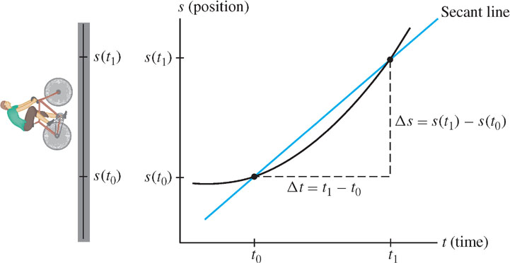
The idea that average velocity converges to instantaneous velocity as we shorten the time interval has a vivid interpretation in terms of secant lines. The term secant line refers to a line through two points on a curve.
Consider the graph of position \(s(t)\) for an object traveling in a straight line (Figure 2.3). The ratio defining average velocity over \([t_0,t_1]\) is nothing more than the slope of the secant line through the points \((t_0,s(t_0))\) and \((t_1,s(t_1))\). For \(t_1 \neq t_0\), \[\text{Average Velocity} = \text{slope of the secant line} = \dfrac{\Delta s}{\Delta t} = \dfrac{s(t_1)-s(t_0)}{t_1-t_0}\]
By interpreting average velocity as a slope, we can visualize what happens as the time interval gets smaller. Figure 2.4 shows the graph of position for the falling stone of Example 1, where \(s(t) = 4.9t^2\). As the time interval shrinks, the secant lines get closer to—and seem to rotate toward—the tangent line at \(t = 0.8\).

And since the secant lines approach the tangent line, the slopes of the secant lines get closer and closer to the slope of the tangent line. In other words, the statement
As the time interval shrinks to zero, the average velocity approaches the instantaneous velocity.
has the graphical interpretation
As the time interval shrinks to zero, the slope of the secant line approaches the slope of the tangent line.
44
We conclude that instantaneous velocity is equal to the slope of the tangent line to the graph of position as a function of time. This conclusion and its generalization to other rates of change are of fundamental importance in differential calculus.
2.1.3 Other Rates of Change
Velocity is only one of many examples of a rate of change. Our reasoning applies to any quantity \(y\) that depends on a variable \(x\) —say, \(y = f(x)\). For any interval \([x_0,x_1]\), we set\[\Delta f = f(x_1) - f(x_0), \quad \Delta x = x_1 - x_0\]
Sometimes, we write \(\Delta y\) and \(\tfrac{\Delta y}{\Delta x}\) instead of \(\Delta f\) and \(\tfrac{\Delta f}{\Delta x}\).
For \(x_1\neq x_0\), the average rate of change of \(y\) with respect to \(x\) over \([x_0,x_1]\) is the ratio
\[\text{Average rate of change} = \frac{\Delta f}{\Delta x} = \frac{f(x_1) - f(x_0)}{x_1 - x_0}\]
The word “instantaneous” is often dropped. When we use the term “rate of change,” it is understood that the instantaneous rate is intended.
The instantaneous rate of change at \(x = x_0\) is the limiting value of the average rates of change. We estimate it by computing the average rate over smaller and smaller intervals.
In Example 1 above, we considered only right-hand intervals \([x_0,x_1]\). In the next example, we compute the average rate of change for intervals lying to both the left and the right of \(x_0\).
EXAMPLE 2 Speed of Sound in Air
The formula \(u=20\sqrt{T}\) provides a good approximation to the speed of sound \(u\) in dry air (in m/s) as a function of air temperature \(T\) (in kelvins). Estimate the instantaneous rate of change of \(u\) with respect to \(T\) when \(T = 273 K\). What are the units of this rate?
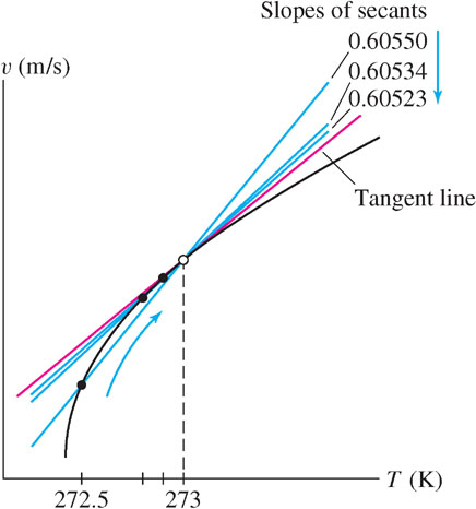
Solution To estimate the instantaneous rate of change at \(T = 273\), we compute the average rate for several intervals lying to the left and right of \(T = 273\). For example, the average rate of change over \([272.5, 273]\) is\[\frac{u(273) - u(272.5)}{273 - 272.5} = \frac{20\sqrt{273} - 20\sqrt{272.5}}{0.5} \approx 0.60550\]
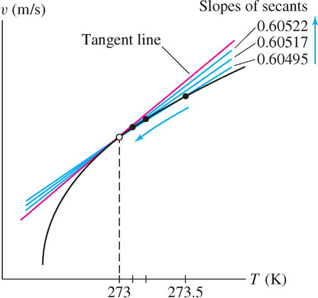
The tables below suggest that the instantaneous rate is approximately 0.605. This is the rate of increase in speed per degree increase in temperature, so it has units of m/s-K, or meters per second per kelvin. The secant lines corresponding to the values in the tables are shown in Figure 2.5 and Figure 2.6.
| Temperature intervals | Average rate of change |
|---|---|
| [272.5, 273] | 0.60550 |
| [272.8, 273] | 0.60534 |
| [272.9, 273] | 0.60528 |
| [272.99, 273] | 0.60523 |
| Temperature intervals | Average rate of change |
|---|---|
| [273, 273.5] | 0.60495 |
| [273, 273.2] | 0.60512 |
| [273, 273.1] | 0.60517 |
| [273, 273.01] | 0.60522 |
Question 2.2 Average Rate of Change Progress Check 1
Find the average rate of change of \(f(x) = -2x^2+x-1\) on the interval \([0,2]\).
| A. |
| B. |
| C. |
| D. |
| E. |
The applet below is designed to give you the opportunity to investigate the average rate of change for a variety of functions.

45
Question 2.3 Average Rate of Change Progress Check 2
Find the average rate of change of \(f(x) = x^2-1\) on the interval \([-1,0.4]\). Give your answer in decimal form. Hint: You can use the applet to do the calculations for you.
To conclude this section, we discuss the case of a simple but important class of functions: For any linear function \(f(x) = mx + b\), the average rate of change over every interval is equal to the slope \(\textstyle m\) (Figure 2.8). We verify as follows: \[\frac{\Delta f}{\Delta x} = \frac{f(x_1) - f(x_0)}{x_1 - x_0} = \frac{(mx_1+b) - (mx_0 + b)}{x_1 - x_0} = \frac{m(x_1 - x_0)}{x_1 - x_0} = m\]
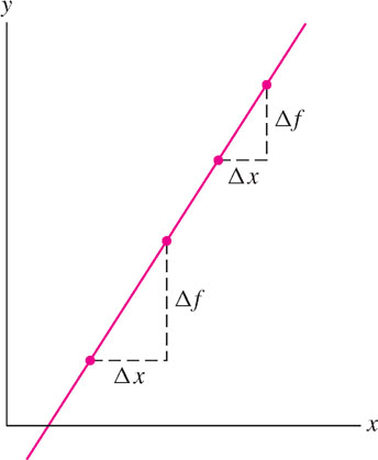
The instantaneous rate of change at \(x = x_0\), which is the limiting value of these average rates, is also equal to \(m\). This makes sense graphically because all secant lines and all tangent lines to the graph of \(f(x)\) coincide with the graph itself.
Question 2.4 Instantaneous Rate of Change Progress Check
What is the instantaneous rate of change of \(f(x)=3x+5\) at \(x_0=1\)?
2.1.4 Summary
- The average rate of change of \(y=f(x)\) over an interval \([x_0,x_1]\) is given by \[\frac{\Delta f}{\Delta x} = \frac{f(x_1) - f(x_0)}{x_1 - x_0}, x_1\neq x_0\]
- The instantaneous rate of change is the limiting value of the average rates of change, if this exists.
- Graphical interpretation: Average rate of change is the slope of the secant line through the points \((x_0,f(x_0))\) and \((x_1,f(x_1))\) on the graph of \(f(x)\).
- Instantaneous rate of change is the slope of the tangent line at \(x_0\).
- To estimate the instantaneous rate of change at \(x=x_0\), compute the average rate of change over several intervals \([x_0,x_1]\) or \([x_1,x_0]\) for \(x_1\) close to \(x_0\).
- The velocity of an object in linear motion is the rate of change of position \(s(t)\).
- Linear function \(f(x) = mx + b\): The average rate of change over every interval and the instantaneous rate of change at every point are equal to the slope \(m\).