2.8 Intermediate Value Theorem
The Intermediate Value Theorem (IVT) says, roughly speaking, that a continuous function cannot skip values, or that the graph of a continuous function is unbroken. Consider a plane that takes off and climbs from 0 to 10,000 meters in 20 minutes. The plane must reach every altitude between 0 and 10,000 meters during this 20-minute interval. Thus, at some moment, the plane’s altitude must have been exactly 8371 meters. Of course, this assumes that the plane’s motion is continuous, so its altitude cannot jump abruptly from, say, 8000 to 9000 meters.
To state this conclusion formally, let \(A(t)\) be the plane’s altitude at time \(t\). The IVT asserts that for every altitude \(M\) between 0 and 10,000, there is a time \(t_0\) between 0 and 20 such that \(A(t_0)=M\). In other words, the graph of \(A(t)\) must intersect the horizontal line \(y=M\) [Figure 2.45(A)].
A proof of the IVT is given in Appendix B.
By contrast, a discontinuous function can skip values. The greatest integer function \(f(x)=[x]\) in Figure 2.45(B) satisfies \([1] = 1\) and \([2] = 2\), but it does not take on the value 1.5 (or any other value between 1 and 2).
107
THEOREM 1 Intermediate Value Theorem
If \(f(x)\) is continuous on a closed interval \([a,b]\) and \(f(a)\neq f(b)\), then for every value \(M\) between \(f(a)\) and \(f(b)\), there exists at least one value \(c\in(a,b)\) such that \(f(c)=M\).
Example 1
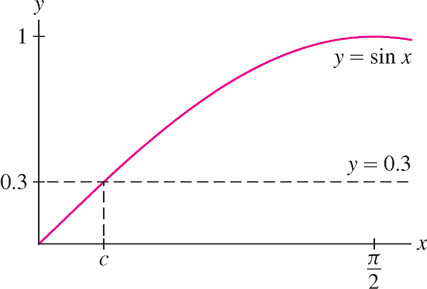
Prove that the equation \(\sin x =0.3\) has at least one solution.
Solution We may apply the IVT because \(\sin x\) is continuous. We choose an interval where we suspect that a solution exists. The desired value \(0.3\) lies between the two function values
\[\sin 0 = 0\text{ and }\sin\frac{\pi}{2} = 1\]
so the interval \([0,{\pi\over 2}]\) will work (Figure 2.46). The IVT tells us that \(\sin x= 0.3\) has at least one solution in \((0,{\pi\over 2})\).
The IVT can be used to show the existence of zeros of functions. If \(f(x)\) is continuous and takes on both positive and negative values —say, \(f(a) < 0\) and \(f(b) > 0\)— then the IVT guarantees that \(f(c) = 0\) for some \(c\) between \(a\) and \(b\). Similarly, the existence of solutions to equations of type \(f(x)=g(x)\) can be established by noting that \(f(x)=g(x)\) is equivalent to \(f(x)-g(x) =0\).
COROLLARY 2 Existence of Zeros
If \(f(x)\) is continuous on \([a,b]\) and if \(f(a)\) and \(f(b)\) are nonzero and have opposite signs, then \(f(x)\) has a zero in \((a,b)\).
A zero or root of a function is a value \(c\) such that \(f(c) = 0\). Sometimes the word “root” is reserved to refer specifically to the zero of a polynomial.
Question 2.25 Intermediate Value Progress Check Question 1
The function \(f(x) =x+e^x\) has one real zero \(x_0\). In which of the following intervals must \(x_0\) lie?
| A. |
| B. |
| C. |
| D. |
We can locate zeros of functions to arbitrary accuracy using the Bisection Method, as illustrated in the next example.
Example 2 The Bisection Method
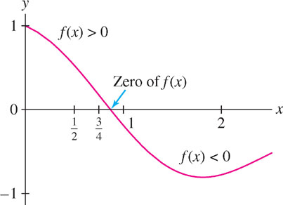
Show that \(f(x) = \cos^2x - 2\sin\frac{x}{4}\) has a zero in \((0, 2)\). Then locate the zero more accurately using the Bisection Method.
Solution Using a calculator, we find that \(f(0)\) and \(f(2)\) have opposite signs:
\[f(0) = 1 > 0 \text{ and }f(2) \approx -0.786 < 0\]
Corollary 2 guarantees that \(f(x) = 0\) has a solution in \((0, 2)\) (Figure 2.47).
Computer algebra systems have built-in commands for finding roots of a function or solving an equation numerically. These systems use a variety of methods, including more sophisticated versions of the Bisection Method. Notice that to use the Bisection Method, we must first find an interval containing a root.
To locate a zero more accurately, divide \([0, 2]\) into two intervals \([0, 1]\) and \([1, 2]\). At least one of these intervals must contain a zero of \(f(x)\). To determine which, evaluate \(f(x)\) at the midpoint \(m=1\). A calculator gives \(f(1)\approx -0.203 < 0\), and since \(f(0)=1\), we see that
\(f(x)\) takes on opposite signs at the endpoints of \([0, 1]\).
Therefore, \((0, 1)\) must contain a zero. We discard \([1, 2]\) because both \(f(1)\) and \(f(2)\) are negative.
The Bisection Method consists of continuing this process until we narrow down the location of the zero to any desired accuracy. In the following table, the process is carried out three times:
108
| Interval | Midpoint of interval | Function values | Conclusion |
|---|---|---|---|
| \([0, 1]\) | \(\frac{1}{2}\) | \(\begin{aligned}f\left(\tfrac{1}{2}\right)&\approx0.521\\ f\left({1}\right)&\approx-0.203\end{aligned}\) | Zero lies in \(\left(\tfrac{1}{2},1\right)\) |
| \([\tfrac{1}{2},1]\) | \(\tfrac{3}{4}\) | \(\begin{aligned}f\left(\tfrac{3}{4}\right)&\approx0.163\\ f\left({1}\right)&\approx-0.203\end{aligned}\) | Zero lies in \(\left(\tfrac{3}{4},1\right)\) |
| \([\tfrac{3}{4},\tfrac{7}{8}]\) | \(\tfrac{7}{8}\) | \(\begin{aligned}f\left(\tfrac{7}{8}\right)&\approx-0.0231\\ f\left(\tfrac{3}{4}\right)&\approx0.163\end{aligned}\) | Zero lies in \(\left(\tfrac{3}{4},\tfrac{7}{8}\right)\) |
We conclude that \(f(x)\) has a zero \(c\) satisfying \(0.75 < c < 0.875\).
CONCEPTUAL INSIGHT
The IVT seems to state the obvious, namely that a continuous function cannot skip values. Yet its proof (given in Appendix B) is subtle because it depends on the completeness property of real numbers. To highlight the subtlety, observe that the IVT is false for functions defined only on the rational numbers. For example, \(f(x)=x^2\) is continuous, but it does not have the intermediate value property if we restrict its domain to the rational numbers. Indeed, \(f(0)=0\) and \(f(2)=4\), but \(f(c)=2\) has no solution for \(c\) rational. The solution \(c=\sqrt{2}\) is “missing” from the set of rational numbers because it is irrational. No doubt the IVT was always regarded as obvious, but it was not possible to give a correct proof until the completeness property was clarified in the second half of the nineteenth century.
2.8.1 Section 2.8 Summary
- The Intermediate Value Theorem (IVT) says that a continuous function cannot skip values, or that the graph of a continuous function is unbroken.
- More precisely, if \(f(x)\) is continuous on \([a,b]\) with \(f(a)\neq f(b)\), and if \(M\) is a number between \(f(a)\) and \(f(b)\), then \(f(c)=M\) for some \(c\in(a,b)\).
- Existence of zeros: If \(f(x)\) is continuous on \([a,b]\) and if \(f(a)\) and \(f(b)\) take opposite signs (one is positive and the other negative), then \(f(c)=0\) for some \(c\in(a,b)\).
- Bisection Method: Assume \(f\) is continuous and that \(f(a)\) and \(f(b)\) have opposite signs, so that \(f\) has a zero in \((a,b)\). Then \(f\) has a zero in \([a,m]\) or \([m,b]\), where \(m=\tfrac{a+b}{2}\) is the midpoint of \([a,b]\). A zero lies in \((a,m)\) if \(f(a)\) and \(f(m)\) have opposite signs and in \((m,b)\) if \(f(m)\) and \(f(b)\) have opposite signs. Continuing the process, we can locate a zero with arbitrary accuracy.