3.4 Rates of Change
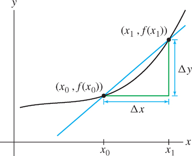
Recall the notation for the average rate of change of a function \(y = f(x)\) over an interval \([x_{0}, x_{1}]\):
\begin{align*} \Delta y &= \text{change in }y &\hspace{-20pt}&= f(x_1)- f(x_0) \\ \Delta x &= \text{change in }x&\hspace{-20pt}&=x_1-x_0 \end{align*} \[\boxed{\text{Average Rate of Change} = \dfrac{\Delta y}{\Delta x} = \dfrac{f(x_1)-f(x_0)}{x_1-x_0}}\]
We usually omit the word “instantaneous” and refer to the derivative simply as the rate of change. This is shorter and also more accurate when applied to general rates, because the term “instantaneous” would seem to refer only to rates with respect to time.
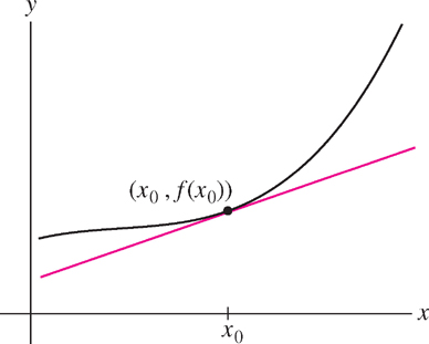
In our prior discussion in Section 2.1, limits and derivatives had not yet been introduced. Now that we have them at our disposal, we can define the instantaneous rate of change of \(y\) with respect to \(x\) at \(x = x_{0}\):
\[\boxed{\text{Instantaneous Rate of Change} = f'(x_0) = \lim\limits_{\Delta x\rightarrow 0}\dfrac{\Delta y}{\Delta x} = \lim\limits_{x_1\rightarrow x_0}\dfrac{f(x_1)-f(x_0)}{x_1-x_0}}\]
Keep in mind the geometric interpretations: The average rate of change is the slope of the secant line (Figure 3.28), and the instantaneous rate of change is the slope of the tangent line (Figure 3.29).
Leibniz notation \(\frac{dy}{dx}\) is particularly convenient because it specifies that we are considering the rate of change of \(y\) with respect to the independent variable \(x\). The rate \(\frac{dy}{dx}\) is measured in units of \(y\) per unit of \(x\). For example, the rate of change of temperature with respect to time has units such as degrees per minute, whereas the rate of change of temperature with respect to altitude has units such as degrees per kilometer.
EXAMPLE 1
| Time | Temperature (°C) |
|---|---|
| 5:42 | -74.7 |
| 6:11 | -71.6 |
| 6:40 | -67.2 |
| 7:09 | -63.7 |
| 7:38 | -59.5 |
| 8:07 | -53 |
| 8:36 | -47.7 |
| 9:05 | -44.3 |
| 9:34 | -42 |
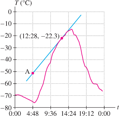
Table 3.2 contains data on the temperature \(T\) on the surface of Mars at Martian time \(t\), collected by the NASA Pathfinder space probe.
(a) Calculate the average rate of change of temperature \(T\) from 6:11 AM to 9:05 AM.
(b) Use Figure 3.30 to estimate the rate of change at \(t = 12:28\)PM.
Solution
(a) The time interval \([6:11, 9:05]\) has length 2 h, 54 min, or \(\Delta t = 2.9 h\). According to Table 1, the change in temperature over this time interval is
\[\Delta T = -44.3 - (-71.6) = 27.3^{\circ}C\]
The average rate of change is the ratio
\[\frac{\Delta T}{\Delta t} = \frac{27.3}{2.9}\approx 9.4^{\circ}C/h\]
151
(b) The rate of change is the derivative \(\frac{\Delta T}{\Delta t}\), which is equal to the slope of the tangent line through the point \((12:28, -22.3)\) in Figure 3.30. To estimate the slope, we must choose a second point on the tangent line. Let’s use the point labeled \(A\), whose coordinates are approximately \((4:48, -51)\). The time interval from \(4:48\)AM to \(12:28\)PM has length 7 h, 40 min, or \(\Delta t = 7.67 h\), and
\[\frac{dT}{dt}=\text{slope of the tangent line}\approx \frac{-22.3-(-51)}{7.67}\approx3.7^{\circ}C/h\]
EXAMPLE 2
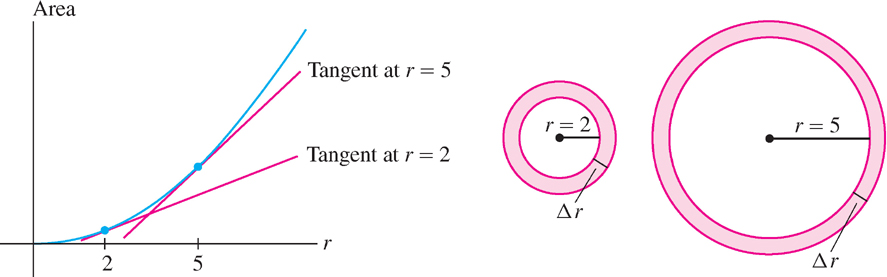
Let \(A = \pi r^{2}\) be the area of a circle of radius \(r\).
(a) Compute \(\frac{dA}{dr}\) at \(r = 2\) and \(r = 5\).
(b) Why is \(\frac{dA}{dr}\) larger at \(r = 5\)?
Solution The rate of change of area with respect to radius is the derivative
\[\frac{dA}{dr} = \frac{d}{dr}(\pi r^2) = 2\pi r\tag{1}\]
By Eq. (1), \(\frac{dA}{dr}\) is equal to the circumference \(2\pi r\). We can explain this intuitively as follows: Up to a small error, the area \( \Delta A\) of the band of width \( \Delta r\) in Figure 3.31 is equal to the circumference \( 2\pi r\) times the width \( \Delta r\). Therefore, \(\Delta A \approx 2\pi r\Delta r\) and
\[\frac{dA}{dr}=\lim\limits_{\Delta r\rightarrow 0}\frac{\Delta A}{\Delta r}=2\pi r\]
The fact that the rate of change of the area is the circumference is quite significant. It can be used in reverse; i.e. knowing the circumference can give you a formula for the area. This is essentially part of the Fundamental Theorem of Calculus that we will discuss in Chapter 5.
(a) We have
\[\frac{dA}{dr}\Bigg|_{r=2}=2\pi(2)\approx12.57\text{ and }\frac{dA}{dr}\Bigg|_{r=5}2\pi(5)\approx31.42\]
(b) The derivative \(\frac{dA}{dr}\) measures how the area of the circle changes when \(r\) increases. Figure 3.31 shows that when the radius increases by \(\Delta r\), the area increases by a band of thickness \(\Delta r\). The area of the band is greater at \(r = 5\) than at \(r = 2\). Therefore, the derivative is larger (and the tangent line is steeper) at \(r = 5\). In general, for a fixed \(\Delta r\), the change in area \(\Delta A\) is greater when \(r\) is larger.
3.4.1 The Effect of a One-Unit Change
For small values of \(h\), the difference quotient is close to the derivative itself:
\[f'(x_0)\approx\frac{f(x_0+h)-f(x_0)}{h}\tag{2}\]
This approximation generally improves as \(h\) gets smaller, but in some applications, the approximation is already useful with \(h = 1\). Setting \(h = 1\) in Eq. (2) gives
\[\boxed{f'(x_0)\approx f(x_0+1)-f(x_0)}\tag{3}\]
In other words, \(f'(x_{0})\) is approximately equal to the change in \(f\) caused by a one-unit change in \(x\) when \(x= x_{0}\).
152
EXAMPLE 3 Stopping Distance
 For speeds \(s\) between 30 and 75 mph, the stopping distance of an automobile after the brakes are applied is approximately \(F(s) = 1.1s + 0.05s^{2} \text{ ft}\). For \(s = 60 \text{ mph}\):
(a) Estimate the change in stopping distance if the speed is increased by 1 mph.
(b) Compare your estimate with the actual increase in stopping distance.
Solution
(a) We have
\begin{align*}F'(s)&=\frac{d}{ds}(1.1s + 0.05s^{2})=1.1 + 0.1s\text{ ft/mph}\\ F'(60)&=1.1+6 = 7.1\text{ ft/mph}\end{align*}
Using Eq. (3), we estimate
\[\underbrace{F(61)-F(60)}_{\scriptscriptstyle\text{Change in stopping distance}}\approx F'(60) = 7.1\text{ ft/mph}\]
Thus, when you increase your speed from 60 to 61 mph, your stopping distance increases by roughly 7 ft.
(b) The actual change in stopping distance is \(F(61) - F(60) = 253.15 - 246 = 7.15\), so the estimate in (a) is fairly accurate.
3.4.2 Marginal Cost in Economics
Although \(C(x)\) is meaningful only when \(x\) is a whole number, economists often treat \(C(x)\) as a differentiable function of \(x\) so that the techniques of calculus can be applied.
Let \(C(x)\) denote the dollar cost (including labor and parts) of producing \(x\) units of a particular product. The number \(x\) of units manufactured is called the production level. To study the relation between costs and production, economists define the marginal cost at production level \(x_{0}\) as the cost of producing one additional unit:
\[\text{Marginal cost} = C(x_{0} + 1) - C(x_{0})\]
In this setting, Eq. (3) usually gives a good approximation, so we take \(C'(x_{0})\) as an estimate of the marginal cost.
EXAMPLE 4 Cost of an Air Flight
Company data suggest that the total dollar cost of a certain flight is approximately \(C(x) = 0.0005x^{3} - 0.38x^{2} + 120x\), where \(x\) is the number of passengers (Figure 3.32).
(a) Estimate the marginal cost of an additional passenger if the flight already has 150 passengers.
(b) Compare your estimate with the actual cost of an additional passenger.
(c) Is it more expensive to add a passenger when \(x = 150\) or when \(x = 200\)?
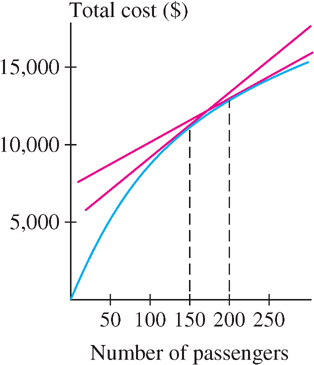
Solution The derivative is \(C'(x) = 0.0015x^{2} - 0.76x + 120\).
(a) We estimate the marginal cost at \(x = 150\) by the derivative
\[C'(150) = 0.0015(150)^{2} - 0.76(150) + 120 = 39.75\]
Thus, it costs approximately $39.75 to add one additional passenger.
(b) The actual cost of adding one additional passenger is
\[C(151) - C(150) \approx 11,177.10 - 11,137.50 = 39.60\]
Our estimate of $39.75 is close enough for practical purposes.
153
(c) The marginal cost at \(x = 200\) is approximately
\[C'(200) = 0.0015(200)^{2} - 0.76(200) + 120 = 28\]
Since \(39.75 > 28\), it is more expensive to add a passenger when \(x = 150\).
3.4.3 Linear Motion
In his famous textbook Lectures on Physics, Nobel laureate Richard Feynman (1918–1988) uses a dialogue to make a point about instantaneous velocity:
Policeman: “My friend, you were going 75 miles an hour.”
Driver: “That’s impossible, sir, I was traveling for only seven minutes.”
Recall that linear motion is motion along a straight line. This includes horizontal motion along a straight highway and vertical motion of a falling object. Let \(s(t)\) denote the position or distance from the origin at time \(t\). Velocity is the rate of change of position with respect to time:
\[v(t)=\text{velocity}=\frac{ds}{dt}\]
The sign of \(v(t)\) indicates the direction of motion. For example, if \(s(t)\) is the height above ground, then \(v(t) > 0\) indicates that the object is rising. Speed is defined as the absolute value of velocity \(|v(t)|\).
Figure 3.33 shows the position of a car as a function of time. Remember that the height of the graph represents the car’s distance from the point of origin. The slope of the tangent line is the velocity. Here are some facts we can glean from the graph:
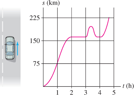
- Speeding up or slowing down? The tangent lines get steeper in the interval \([0, 1]\), so the car was speeding up during the first hour. They get flatter in the interval \([1, 2]\), so the car slowed down in the second hour.
- Standing still The graph is horizontal over \([2, 3]\) (perhaps the driver stopped at a restaurant for an hour).
- Returning to the same spot The graph rises and falls in the interval \([3, 4]\), indicating that the driver returned to the restaurant (perhaps she left her cell phone there).
- Average velocity The graph rises more over \([0, 2]\) than over \([3, 5]\), so the average velocity was greater over the first two hours than over the last two hours.
EXAMPLE 5
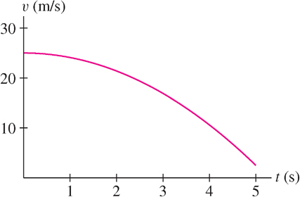
A truck enters the off-ramp of a highway at \(t = 0\). Its position after \(t\) seconds is \(s(t) = 25t - 0.3t^{3}\text{ m}\) for \(0 \leq t \leq 5\).
(a) How fast is the truck going at the moment it enters the off-ramp?
(b) Is the truck speeding up or slowing down?
Solution The truck’s velocity at time \(t\) is \(v(t)=\frac{d}{dt}(25t-0.3t^3)=25-0.9t^2\).
(a) The truck enters the off-ramp with velocity \(v(0) = 25\text{ m/s}\).
(b) Since \(v(t) = 25 - 0.9t^{2}\) is decreasing (Figure 3.34), the truck is slowing down.
3.4.4 Motion Under the Influence of Gravity
Galileo discovered that the height \(s(t)\) and velocity \(v(t)\) at time \(t\) (seconds) of an object tossed vertically in the air near the earth’s surface are given by the formulas
Galileo’s formulas are valid only when air resistance is negligible. We assume this to be the case in all examples.
\[\boxed{s(t)=s_0+v_0t-\dfrac{1}{2}gt^2}\tag{4}\]
The constants \(s_{0}\) and \(v_{0}\) are the initial values:
- \(s_{0} = s(0)\), the position at time \(t = 0\).
- \(v_{0} = v(0)\), the velocity at \(t = 0\).
- \(-g\) is the acceleration due to gravity on the surface of the earth (negative because the up direction is positive), where
154
A simple observation enables us to find the object’s maximum height. Since velocity is positive as the object rises and negative as it falls back to earth, the object reaches its maximum height at the moment of transition, when it is no longer rising and has not yet begun to fall. At that moment, its velocity is zero. In other words, the maximum height is attained when \(v(t) = 0\). At this moment, the tangent line to the graph of \(s(t)\) is horizontal (Figure 3.35).
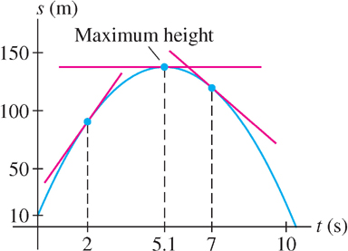
EXAMPLE 6 Finding the Maximum Height
A stone is shot with a slingshot vertically upward with an initial velocity of 50 m/s from an initial height of 10 m.
(a) Find the velocity at \(t = 2\) and at \(t = 7\). Explain the change in sign.
(b) What is the stone’s maximum height and when does it reach that height?
Galileo’s formulas:
\begin{align*}s(t)&=s_0+v_0t-\dfrac{1}{2}gt^2\\ v(t)&=\dfrac{ds}{dt}=v_0 - gt\end{align*}
Solution Apply Eq. (4) with \(s_{0} = 10\), \(v_{0} = 50\), and \(g = 9.8\):
\[s(t)=10+50t-4.9t^2\text{ and }v(t) = 50 -9.8t\]
(a) Therefore,
\[v(2) = 50 -9.8(2) = 30.4\text{ m/s and }v(7)=50-9.8(7)=-18.6\text{ m/s}\]
At \(t = 2\), the stone is rising and its velocity \(v(2)\) is positive (Figure 3.35). At \(t = 7\), the stone is already on the way down and its velocity \(v(7)\) is negative.
(b) Maximum height is attained when the velocity is zero, so we solve
\[v(t) = 50-9.8t = 0\implies t=\frac{50}{9.8}\approx5.1\text{ s}\]
The stone reaches maximum height at \(t = 5.1\) s. Its maximum height is
\[s(5.1) = 10 + 50(5.1) - 4.9(5.1)^{2} \approx 137.6\text{ m}\]
In the previous example, we specified the initial values of position and velocity. In the next example, the goal is to determine initial velocity.
EXAMPLE 7 Finding Initial Conditions
How important are units? In September 1999, the $125 million Mars Climate Orbiter spacecraft burned up in the Martian atmosphere before completing its scientific mission. According to Arthur Stephenson, NASA chairman of the Mars Climate Orbiter Mission Failure Investigation Board, 1999, “The ‘root cause’ of the loss of the spacecraft was the failed translation of English units into metric units in a segment of ground-based, navigation-related mission software.”
What initial velocity \(v_{0}\) is required for a bullet, fired vertically from ground level, to reach a maximum height of 2 km?
Solution We need a formula for maximum height as a function of initial velocity \(v_{0}\). The initial height is \(s_{0} = 0\), so the bullet’s height is \(s(t)=v_0t-\frac{1}{2}gt^2\) by Galileo’s formula. Maximum height is attained when the velocity is zero:
\[v(t)=v_0-gt=0\implies t=\frac{v_0}{g}\]
The maximum height is the value of \(s(t)\) at \(t = v_{0}/g\):
\[s\left(\frac{v_0}{g}\right)=v_0\left(\frac{v_0}{g}\right)-\frac{1}{2}g\left(\frac{v_0}{g}\right)^2 = \frac{v_0^2}{g}- \frac{v_0^2}{2g}=\frac{v_0^2}{2g}\]
Now we can solve for \(v_{0}\) using the value \(g = 9.8\text{ m/s}^{2}\) (note that \(2 km = 2000 m\)).
In Eq. (5), distance must be in meters because our value of \(g\) has units of \(\text{m/s}^{2}\).
\[\text{Maximum height} = \frac{v_0^2}{2g}= \frac{v_0^2}{2(9.8)}= 2000\text{ m}\tag{5}\]
This yields \(v_0=\sqrt{(2)(9.8)2000}\approx 198\text{ m/s}\). In reality, the initial velocity would have to be considerably greater to overcome air resistance.
155
HISTORICAL PERSPECTIVE
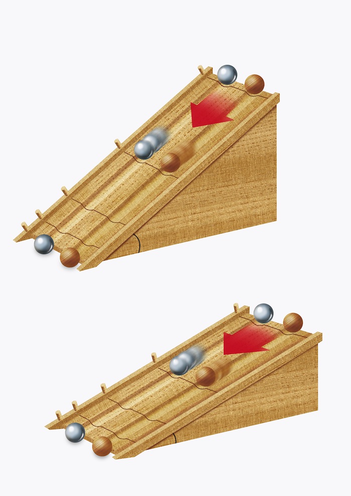
Galileo Galilei (1564–1642) discovered the laws of motion for falling objects on the earth’s surface around 1600. This paved the way for Newton’s general laws of motion. How did Galileo arrive at his formulas? The motion of a falling object is too rapid to measure directly, without modern photographic or electronic apparatus. To get around this difficulty, Galileo experimented with balls rolling down an incline (Figure 3.37). For a sufficiently flat incline, he was able to measure the motion with a water clock and found that the velocity of the rolling ball is proportional to time. He then reasoned that motion in free-fall is just a faster version of motion down an incline and deduced the formula \(v(t) = -gt\) for falling objects (assuming zero initial velocity).
Prior to Galileo, and due to Aristotle, it had been assumed incorrectly that heavy objects fall more rapidly than lighter ones. Galileo realized that this was not true (as long as air resistance is negligible), and indeed, the formula \(v(t) = -gt\) shows that the velocity depends on time but not on the weight of the object. Interestingly, 300 years later, another great physicist, Albert Einstein, was deeply puzzled by Galileo’s discovery that all objects fall at the same rate regardless of their weight. He called this the Principle of Equivalence and sought to understand why it was true. In 1916, after a decade of intensive work, Einstein developed the General Theory of Relativity, which finally gave a full explanation of the Principle of Equivalence in terms of the geometry of space and time.
3.4.5 Section 3.4 Summary
- The (instantaneous) rate of change of \(y = f(x)\) with respect to \(x\) at \(x = x_{0}\) is defined as the derivative
\[f'(x_0) = \lim\limits_{\Delta x\rightarrow 0}\frac{\Delta y}{\Delta x} = \lim\limits_{x_1\rightarrow x_0}\frac{f(x_1)-f(x_0)}{x_1-x_0}\]
- The rate \(\frac{dy}{dx}\) is measured in units of \(y\) per unit of \(x\).
- For linear motion, velocity \(v(t)\) is the rate of change of position \(s(t)\) with respect to time—that is, \(v(t) = s'(t)\).
- In some applications, \(f'(x_{0})\) provides a good estimate of the change in \(f\) due to a one-unit increase in \(x\) when \(x = x_{0}\):
\[f'(x_{0}) \approx f(x_{0} + 1) - f(x_{0})\]
- Marginal cost is the cost of producing one additional unit. If \(C(x)\) is the cost of producing \(x\) units, then the marginal cost at production level \(x_{0}\) is \(C(x_{0} + 1) - C(x_{0})\). The derivative \(C'(x_{0})\) is often a good estimate for marginal cost.
- Galileo’s formulas for an object rising or falling under the influence of gravity near the earth’s surface (\(s_{0} = \text{initial position}, v_{0} = \text{initial velocity}\)):
\[s(t) = s_0+v_0y-\frac{1}{2}gt^2\text{ and }v(t) = v_0-gt\]
where \(g \approx 9.8 m/s^{2}\), or \(g \approx 32\text{ ft/s}^{2}\). Maximum height is attained when \(v(t) = 0\).