4.1 Linear Approximation and Applications
In some situations we are interested in determining the “effect of a small change.” For example:
- How does a small change in angle affect the distance of a basketball shot? (Exercise 39)
- How are revenues at the box office affected by a small change in ticket prices? (Exercise 29)
- The cube root of 27 is 3. How much larger is the cube root of 27.2? (Exercise 7)
In each case, we have a function \(f(x)\) and we’re interested in the change
\[ \boxed{\Delta f = f(a+\Delta x) - f(a)} \]
where \(\Delta x\) is small. The Linear Approximation uses the derivative to estimate \(\Delta f\) without computing it exactly. By definition, the derivative is the limit
\[ f'(a) = \lim\limits_{\Delta x\rightarrow 0}\frac{f(a+\Delta x) - f(a)}{\Delta x} = \lim\limits_{\Delta x\rightarrow 0}\frac{\Delta f}{\Delta x} \]
So when \(\Delta x\) is small, we have \(\frac{\Delta f}{\Delta x} \approx f'(a)\), and thus,
\[ \Delta f \approx f'(a)\Delta x \]
![]() REMINDER The notation \(\approx\) means “approximately equal to.” The accuracy of the Linear Approximation is discussed at the end of this section.
REMINDER The notation \(\approx\) means “approximately equal to.” The accuracy of the Linear Approximation is discussed at the end of this section.
Linear Approximation of Δf
If \(f\) is differentiable at \(x = a\) and \(\Delta x\) is small, then
\[ \boxed{\Delta f \approx f'(a)\Delta x}\tag{1} \]
where \(\Delta f = f(a + \Delta x) - f(a)\).
Keep in mind the different roles played by \(\Delta f\) and \(f'(a)\Delta x\). The quantity of interest is the actual change \(\Delta f\). We estimate it by \(f'(a) \Delta x\). The Linear Approximation tells us that up to a small error, \(\Delta f\) is directly proportional to \(\Delta x\) when \(\Delta x\) is small.
208
GRAPHICAL INSIGHT
The Linear Approximation is sometimes called the tangent line approximation. Why? Observe in Figure 4.1 that \(\Delta f\) is the vertical change in the graph from \(x = a\) to \(x = a + \Delta x\). For a straight line, the vertical change is equal to the slope times the horizontal change \(\Delta x\), and since the tangent line has slope \(f'(a)\), its vertical change is \(f'(a)\Delta x\). So the Linear Approximation approximates \(\Delta f\) by the vertical change in the tangent line. When \(\Delta x\) is small, the two quantities are nearly equal.
EXAMPLE 1
Linear Approximation:
\[ \Delta f \approx f'(a)\Delta x \]
where\( \Delta f = f(a + \Delta x) - f(a)\)
Use the Linear Approximation to estimate \(\frac{1}{10.2} - \frac{1}{10}\). How accurate is your estimate?
Solution We apply the Linear Approximation to \(f(x)=\frac{1}{x}\) with \(a = 10\) and \(\Delta x = 0.2\):
\[ \Delta f = f(10.2) - f(10) = \frac{1}{10.2} - \frac{1}{10} \]
We have \(f'(x) = -x^{-2}\)and\( f'(10) = -0.01\), so \(\Delta f\) is approximated by
\[ f'(10)\Delta x = (-0.01)(0.2) = -0.002 \]
In other words,
\[ \frac{1}{10.2} - \frac{1}{10} \approx -0.002 \]
The error in the Linear Approximation is the quantity
\[ \text{Error} = |\Delta f - f'(a)\Delta x| \]
A calculator gives the value \(\frac{1}{10.2} - \frac{1}{10} \approx -0.00196\) and thus our error is less than \(10^{-4}\):
\[ \text{Error} \approx |-0.00196 -(-0.002)| = 0.00004 < 10^{-4} \]
Question 4.1 Linear Approximation Progress Check Question 1
Use the linear approximation to estimate \( \sin(.03)-\sin(0)= \sin(.03)-0= \sin(.03)\)
Differential Notation
The Linear Approximation to \(y = f(x)\) is often written using the “differentials” \(dx\) and \(dy\). In this notation, \(dx\) is used instead of \(\Delta x\) to represent the change in \(x\), and \(dy\) is the corresponding vertical change in the tangent line:
\[ \boxed{dy = f'(a)dx}\tag{2} \]
Let \(\Delta y = f(a + dx) - f(a)\). Then the Linear Approximation says
\[\boxed{\Delta y\approx dy}\tag{3}\]
This is simply another way of writing \(\Delta f \approx f'(a)\Delta x\).
EXAMPLE 2 Differential Notation
Approximately how much larger is \(\sqrt[3]{8.1}\) than \(\sqrt[3]{8} = 2\)?
Solution We are interested in \(\sqrt[3]{8.1} - \sqrt[3]{8}\), so we apply the Linear Approximation to \(f(x) = x^{\frac{1}{3}}\) with \(a = 8\) and change \(\Delta x = dx = 0.1\).
209
Step 1. Write out \(\Delta y\).
\[ \Delta y = f(a+dx) - f(a) =\sqrt[3]{8+0.1} - \sqrt[3]{8} = \sqrt[3]{8.1} - 2 \]
Step 2. Compute \(dy\).
\[ f'(x) = \frac{1}{3}x^{-\frac{2}{3}}\text{ and }f'(8)=\left(\frac{1}{3}\right)8^{-\frac{2}{3}} = \left(\frac{1}{3}\right)\left(\frac{1}{4}\right)=\frac{1}{12} \]
Therefore, \(dy = f'(8)dx =\frac{1}{12}(0.1)\approx 0.0083\).
Step 3. Use the Linear Approximation.
\[ \Delta y\approx dy\implies \sqrt[3]{8.1} - 2 \approx 0.0083 \]
Thus \(\sqrt[3]{8.1}\) is larger than \(\sqrt[3]{8}\) by approximately 0.0083, and \(\sqrt[3]{8.1}\approx2.0083\).
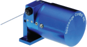
When engineers need to monitor the change in position of an object with great accuracy, they may use a cable position transducer (Figure 4.2). This device detects and records the movement of a metal cable attached to the object. Its accuracy is affected by changes in temperature because heat causes the cable to stretch. The Linear Approximation can be used to estimate these effects.
EXAMPLE 3 Thermal Expansion
A thin metal cable has length \(L = 12\text{ cm}\) when the temperature is \(T = 21^\circ\text{C}\). Estimate the change in length when \(T\) rises to 24°C, assuming that
\[ \frac{dL}{dT} = kL\tag{4} \]
where \(k = 1.7 \times10^{-5}(^\circ\text{C})^{-1}\) (\(k\) is called the coefficient of thermal expansion).
Solution How does the Linear Approximation apply here? We will use the differential \(dL\) to estimate the actual change in length \(\Delta L\) when \(T\) increases from 21° to 24°—that is, when \(dT = 3^\circ\). By Eq. (2), the differential \(dL\) is
\[ dL = \left(\frac{dL}{dT}\right)dT \]
By Eq. (4), since \(L = 12\),
\[ \left.\frac{dL}{dT}\right|_{L=12} = k L = (1.7 \times10^{-5})(12) \approx 2\times 10^{-4}\text{ cm/\(^\circ\)C} \]
The Linear Approximation \(\Delta L \approx dL\) tells us that the change in length is approximately
\[ \Delta L \approx\underbrace{\left(\frac{dL}{dT}\right)dT}_{dL}\approx(2\times 10^{-4})(3) = 6\times 10^{-4}\text{ cm} \]
Suppose that we measure the diameter D of a circle and use this result to compute the area of the circle. If our measurement of D is inexact, the area computation will also be inexact. What is the effect of the measurement error on the resulting area computation? This can be estimated using the Linear Approximation, as in the next example.
EXAMPLE 4 Effect of an Inexact Measurement
The Bonzo Pizza Company claims that its pizzas are circular with diameter 50 cm (Figure 4.3).

(a) What is the area of the pizza?
(b) Estimate the quantity of pizza lost or gained if the diameter is off by at most 1.2 cm.
210
Solution First, we need a formula for the area \(A\) of a circle in terms of its diameter \(D\). Since the radius is \(r = \frac{D}{2}\), the area is
\[ A(D) = \pi r^2 = \pi\left(\frac{D}{2}\right)^2 = \frac{\pi}{4}D^2 \]
(a) If \(D = 50\text{ cm}\), then the pizza has area \(A(50) = \left(\frac{\pi}{4}\right)(50)^2\approx1963.5\text{ cm}^2\).
In this example, we interpret \(\Delta A\) as the possible error in the computation of \(A(D)\). This should not be confused with the error in the Linear Approximation. This latter error refers to the accuracy in using \(A'(D) \Delta D\) to approximate \(\Delta A\).
(b) If the actual diameter is equal to \(50 + \Delta D\), then the loss or gain in pizza area is \(\Delta A = A(50 + \Delta D) - A(50)\). Observe that \(A'(D) = \frac{\pi}{2}D\) and \(A'(50) = 25\pi \approx 78.5\text{ cm}\), so the Linear Approximation yields
\[ \Delta A = A(50 + \Delta D) - A(50) \approx A'(D)\Delta D \approx (78.5) \Delta D \]
Because \(\Delta D\) is at most \(\pm 1.2 \text{ cm}\), the loss or gain in pizza is no more than around
\[ \Delta A \approx \pm (78.5)(1.2) \approx \pm 94.2\text{ cm}^{2} \]
This is a loss or gain of approximately \(4.8\%\).
4.1.1 Linearization
To approximate the function \(f(x)\) itself rather than the change \(\Delta f\), we use the linearization \(L(x)\) “centered at \(x = a\),” defined by
\[ L(x) = f'(a)(x - a) + f(a) \]
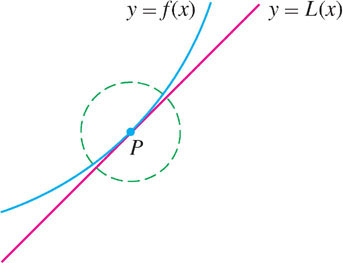
Notice that \(y = L(x)\) is the equation of the tangent line at \(x = a\) (Figure 4.4). If \(f(x)\) is differentiable at \(x=a\), then for values of \(x\) close to \(a\), \(L(x)\) provides a good approximation to \(f(x)\).
Approximating f(x) by Its Linearization
If \(f\) is differentiable at \(x = a\) and \(x\) is close to \(a\), then
\[ \boxed{f(x)\approx L(x) = f'(a)(x - a) + f(a)} \]
CONCEPTUAL INSIGHT
Keep in mind that the linearization and the Linear Approximation are two ways of saying the same thing. Indeed, when we apply the linearization with \(x = a + \Delta x\) and re-arrange, we obtain the Linear Approximation:
\begin{align*} f(x)&\approx f(a) + f'(a)(x-a)\\ f(a + \Delta x) &\approx f(a) + f'(a)\Delta x\quad(\text{since }\Delta x = x-a)\\ f(a + \Delta x) - f(a)&\approx f'(a)\Delta x \end{align*}
EXAMPLE 5
Compute the linearization of \(f(x) = \sqrt{x}e^{x-1}\) centered at \(a = 1\).
Solution By the Product Rule:
\begin{gather*} f'(x) = x^{\frac{1}{2}}e^{x-1} + \frac{1}{2}x^{-\frac{1}{2}}e^{x-1} = \left(x^{\frac{1}{2}} + \frac{1}{2}x^{-\frac{1}{2}}\right)e^{x-1}\\ f(1) = \sqrt1e^0=1\quad f'(1)=\left(1+\frac{1}{2}\right)e^0 = \frac{3}{2} \end{gather*}
Therefore, the linearization at \(a = 1\) is
\[ L(x) = f(1) + f'(1)(x-1) = 1 + \frac{3}{2}(x-1)=\frac{3}{2}x - \frac{1}{2} \]
Question 4.2 Linearization Progress Check 2
Find the linearization \(L(x)\) of \(f(x) = 2x \cos x+1\) at \(x=0\). Give your answer in the form L=mx+b, NO SPACES.
211
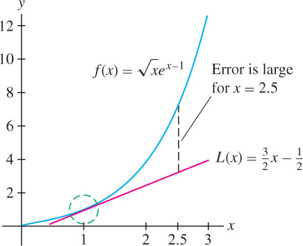
The linearization can be used to approximate function values. The following table compares values of the linearization to values obtained from a calculator for the function \(f(x) = \sqrt{x}e^{x-1}\) in the previous example. Note that the error is large for \(x = 2.5\), as expected, because 2.5 is not close to the center \(a = 1\) (Figure 4.5).
| \(x\) | \(\sqrt{x}e^{x-1}\) | Linearization at \(a = 1\): \(L(x) = \frac{3}{2}x - \frac{1}{2}\) | Calculator | Error |
|---|---|---|---|---|
| \(1.1\) | \(\sqrt{1.1}e^{0.1}\) | \(L(1.1) = \frac{3}{2}(1.1) - \frac{1}{2} = 1.15\) | \(1.15911\) | \(10^{-2}\) |
| \(0.999\) | \(\sqrt{0.999}e^{-0.001}\) | \(L(0.999) = \frac{3}{2}(0.999) - \frac{1}{2} = 0.9985\) | \(0.998501\) | \(10^{-6}\) |
| \(2.5\) | \(\sqrt{2.5}e^{1.5}\) | \(L(2.5) = \frac{3}{2}(2.5) - \frac{1}{2} = 3.75\) | \(7.086\) | \(3.84\) |
In the next example, we compute the percentage error, which is often more important than the error itself. By definition,
\[ \boxed{\text{Percentage error}=\left|\dfrac{\text{error}}{\text{actual value}}\right|\times100\%} \]
EXAMPLE 6
Estimate \(\tan(\frac{\pi}{4}+0.02)\) and compute the percentage error.
Solution We find the linearization of \(f(x)=\tan x\) at \(a=\frac{\pi}{4}\):
\begin{gather*} f\left(\frac{\pi}{4}\right) = \tan\left(\frac{\pi}{4}\right) = 1\quad f'\left(\frac{\pi}{4}\right)=\sec^2\left(\frac{\pi}{4}\right) = (\sqrt{2})^2=2\\ L(x) = f\left(\frac{\pi}{4}\right) + f'\left(\frac{\pi}{4}\right)\left(x-\frac{\pi}{4}\right) = 1 + 2\left(x-\frac{\pi}{4}\right) \end{gather*}
At \(x=\frac{\pi}{4}+0.02\), the linearization yields the estimate
\[ \tan\left(\frac{\pi}{4}+0.02\right)\approx L\left(\frac{\pi}{4}+0.02\right) = 1 + 2(0.02) = 1.04 \]
A calculator gives \(\tan\left(\frac{\pi}{4}+0.02\right)\approx1.0408\), so
\[ \text{Percentage error}\approx\left|\frac{1.0408 - 1.04}{1.0408}\times 100 \approx 0.08\%\right| \]
4.1.2 The Size of the Error
The examples in this section may have convinced you that the Linear Approximation yields a good approximation to \(\Delta f\) when \(\Delta x\) is small, but if we want to rely on the Linear Approximation, we need to know more about the size of the error:
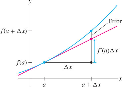
\[ E = \text{Error} = |\Delta f - f'(a)\Delta x| \]
Remember that the error \(E\) is simply the vertical gap between the graph and the tangent line (Figure 4.6). In Section 10.7, we will prove the following Error Bound:
\[ \boxed{E\leq \dfrac{1}{2}K(\Delta x)^2}\tag{5} \]
where \(K\) is the maximum value of \(|f''(x)|\) on the interval from \(a\) to \(a + \Delta x\).
212
Error Bound:
\[ \boxed{E\leq \dfrac{1}{2}K(\Delta x)^2}\tag{5} \]
where \(K\) is the max of \(|f''|\) on the interval \([a, a + \Delta x]\).
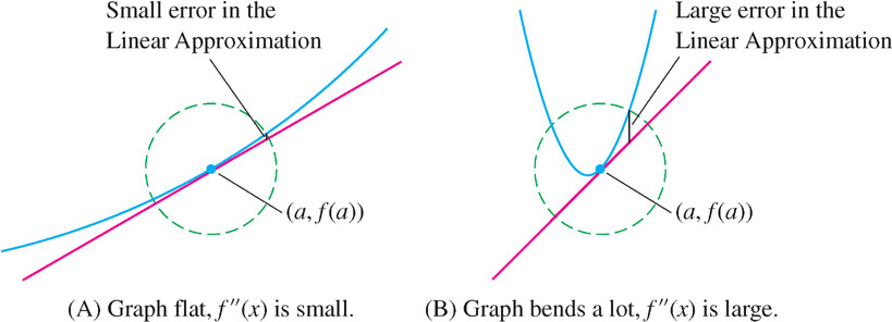
The Error Bound tells us two important things. First, it says that the error is small when the second derivative (and hence \(K\)) is small. This makes sense, because \(f''(x)\) measures how quickly the tangent lines change direction. When \(|f''(x)|\) is smaller, the graph is flatter and the Linear Approximation is more accurate over a larger interval around \(x = a\) (compare the graphs in Figure 4.7).
Second, the Error Bound tells us that the error is of order two
4.1.3 Section 4.1 Summary
- Let \(\Delta f = f(a + \Delta x) - f(a)\). The Linear Approximation is the estimate
\[ \boxed{\Delta f\approx f'(a)\Delta x\quad\text{(for \(\Delta x\) small)}} \]
- Differential notation: \(dx\) is the change in \(x\), \(dy = f'(a)dx\), \(\Delta y = f(a + dx) - f(a)\). In this notation, the Linear Approximation reads
\[ \boxed{\Delta y\approx dy\quad\text{(for \(dx\) small)}} \]
- The linearization of \(f(x)\) at \(x = a\) is the function
\[ \boxed{L(x) = f'(a)(x-a) + f(a)} \]
- The Linear Approximation is equivalent to the approximation
\[ \boxed{f(x)\approx L(x)\quad\text{(for \(x\) close to \(a\))}} \]
- The error in the Linear Approximation is the quantity
\[ \text{Error} = \left|\Delta f - f'(a)\Delta x\right| \]
In many cases, the percentage error is more important than the error itself:
\[ \text{Percentage error} = \left|\frac{\text{error}}{\text{actual value}}\right|\times100\% \]
213