4.2 Extreme Values
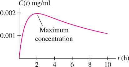
In many applications it is important to find the minimum or maximum value of a function \(f(x)\). For example, a physician needs to know the maximum drug concentration in a patient’s bloodstream when a drug is administered. This amounts to finding the highest point on the graph of \(C(t)\), the concentration at time \(t\) (Figure 4.8).
We refer to the maximum and minimum values (max and min for short) as extreme values or extrema (singular: extremum) and to the process of finding them as optimization. Sometimes, we are interested in finding the min or max for \(x\) in a particular interval \(I\), rather than on the entire domain of \(f(x)\).
Often, we drop the word “absolute” and speak simply of the min or max on an interval \(I\). When no interval is mentioned, it is understood that we refer to the extreme values on the entire domain of the function.
DEFINITION Extreme Values on an Interval
Let \(f(x)\) be a function on an interval \(I\) and let \(d \in I\). We say that \(f(d)\) is the
- Absolute minimum of \(f(x)\) on I if \(f(d) \leq f(x)\) for all \(x \in I\).
- Absolute maximum of \(f(x)\) on \(I\) if \(f(d) \geq f(x)\) for all \(x \in I\).
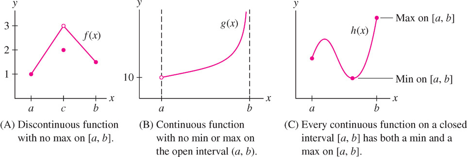
Does every function have a minimum or maximum value? Clearly not, as we see by taking \(f(x) = x\). Indeed, \(f(x) = x\) increases without bound as \(x \rightarrow \infty \) and decreases without bound as \(x \rightarrow -\infty \). In fact, extreme values do not always exist even if we restrict ourselves to an interval \(I\). Figure 4.9 illustrates what can go wrong if \(I\) is open or \(f\) has a discontinuity.
- Discontinuity: (A) shows a discontinuous function with no maximum value. The values of \(f(x)\) get arbitrarily close to 3 from below, but 3 is not the maximum value because \(f(x)\) never actually takes on the value 3.
216
- Open interval: In (B), \(g(x)\) is defined on the open interval \((a, b)\). It has no max because it tends to \(\infty \) on the right, and it has no min because it tends to 10 on the left without ever reaching this value.
Fortunately, our next theorem guarantees that extreme values exist when the function is continuous and \(I\) is closed [Figure 4.9(C)].
![]() REMINDER A closed, bounded interval is an interval \(I = [a, b]\) (endpoints included), where \(a\) and \(b\) are both finite. Often, we drop the word “bounded” and refer to \(I\) more simply as a closed interval. An open interval \((a, b)\) (endpoints not included) may have one or two infinite endpoints.
REMINDER A closed, bounded interval is an interval \(I = [a, b]\) (endpoints included), where \(a\) and \(b\) are both finite. Often, we drop the word “bounded” and refer to \(I\) more simply as a closed interval. An open interval \((a, b)\) (endpoints not included) may have one or two infinite endpoints.
THEOREM 1 Existence of Extrema on a Closed Interval
A continuous function \(f(x)\) on a closed (bounded) interval \(I = [a, b]\) takes on both a minimum and a maximum value on \(I\).
CONCEPTUAL INSIGHT
Why does Theorem 1 require a closed interval? Think of the graph of a continuous function as a string. If the interval is closed, the string is pinned down at the two endpoints and cannot fly off to infinity (or approach a min/max without reaching it) as in Figure 4.9(B). Intuitively, therefore, it must have a highest and lowest point. However, a rigorous proof of Theorem 1 relies on the completeness property of the real numbers (see Appendix D).
4.2.1 Local Extrema and Critical Points
We focus now on the problem of finding extreme values. A key concept is that of a local minimum or maximum.
When we get to the top of a hill in an otherwise flat region, our altitude is at a local maximum, but we are still far from the point of absolute maximum altitude, which is located at the peak of Mt. Everest. That’s the difference between local and absolute extrema.
Adapted from “Stories About Maxima and Minima,” V. M. Tikhomirov, AMS (1990)
DEFINITION Local Extrema
We say that \(f(x)\) has a
- Local minimum at \(x = c\) if \(f(c)\) is the minimum value of \(f\) on some open interval (in the domain of \(f\)) containing \(c\).
- Local maximum at \(x = c\) if \(f(c)\) is the maximum value of \(f(x)\) on some open interval (in the domain of \(f\)) containing \(c\).
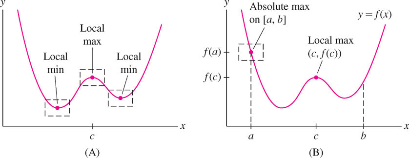
A local max occurs at \(x = c\) if \((c, f(c))\) is the highest point on the graph within some small box [Figure 4.10(A)]. Thus, \(f(c)\) is greater than or equal to all other nearby values, but it does not have to be the absolute maximum value of \(f(x)\). Local minima are similar. Figure 4.10(B) illustrates the difference between local and absolute extrema: \(f(a)\) is the absolute max on \([a, b]\) but is not a local max because \(f(x)\) takes on larger values to the left of \(x = a\).
217
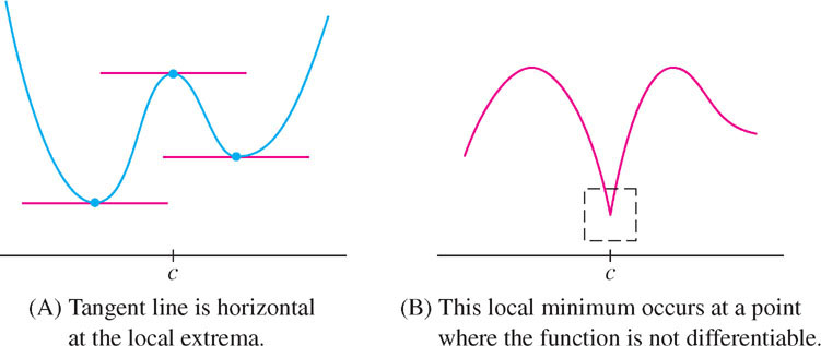
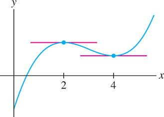
How do we find the local extrema? The crucial observation is that the tangent line at a local min or max is horizontal [Figure 4.11(A)]. In other words, if \(f(c)\) is a local min or max, then \(f'(c) = 0\). However, this assumes that \(f(x)\) is differentiable. Otherwise, the tangent line may not exist, as in Figure 4.11(B). To take both possibilities into account, we define the notion of a critical point.
DEFINITION Interior Point
A point \(c\) in the domain of a function \(f\) is an interior point if there is an open interval containing \(c\) which is also in the domain of \(f\).
DEFINITION Critical Point
An interior point \(c\) in the domain of a function \(f\) is called a critical point if either \(f′(c) = 0\) or \(f′(c)\) does not exist.
EXAMPLE 1
Find the critical points of \(f(x) = x^{3} - 9x^{2} + 24x - 10\).
Solution The function \(f(x)\) is differentiable everywhere (Figure 4.12), so the critical points are the solutions of \(f'(x) = 0\):
\begin{align*} f'(x) = 3x^2 - 18x +24 &=3(x^2-6x+8)\\ &=3(x-2)(x-4) = 0 \end{align*}
The critical points are the roots \(c = 2\) and \(c = 4\).
Question 4.3 Extrema Progress Check 1
Find all critical points of \(\displaystyle f(x)=xe^x\)
| A. |
| B. |
| C. |
| D. |
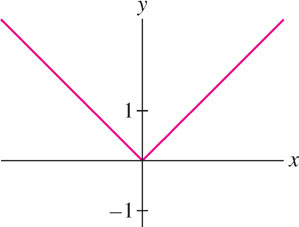
EXAMPLE 2 Nondifferentiable Function
Find the critical points of \(f(x) = |x|\).
Solution
The next theorem tells us that we can find local extrema by solving for the critical points. It is one of the most important results in calculus.
218
THEOREM 2 Fermat’s Theorem on Local Extrema
If \(f(c)\) is a local min or max, then \(c\) is a critical point of \(f(x)\).
Proof
Suppose that \(f(c)\) is a local minimum (the case of a local maximum is similar). If \(f'(c)\) does not exist, then \(c\) is a critical point and there is nothing more to prove. So assume that \(f'(c)\) exists. We must then prove that \(f'(c) = 0\).
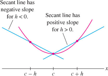
Because \(f(c)\) is a local minimum, we have \(f(c + h) \geq f(c)\) for all sufficiently small \(h \neq 0\). Equivalently, \(f(c + h) - f(c) \geq 0\). Now divide this inequality by \(h\):
\begin{align*} \frac{f(c+h)-f(c)}{h}\geq0&\quad\text{if }h>0\tag{1}\\ \frac{f(c+h)-f(c)}{h}\leq0&\quad\text{if }h<0\tag{2} \end{align*}
Figure 4.14 shows the graphical interpretation of these inequalities. Taking the one-sided limits of both sides of (1) and (2), we obtain
\begin{align*} f'(c)&=\lim\limits_{h\rightarrow 0^+}\frac{f(c+h)-f(c)}{h}\geq\lim\limits_{h\rightarrow 0^+}0=0\\ f'(c)&=\lim\limits_{h\rightarrow 0^-}\frac{f(c+h)-f(c)}{h}\leq\lim\limits_{h\rightarrow 0^-}0=0 \end{align*}
Thus \(f'(c) \geq 0\) and \(f'(c) \leq 0\). The only possibility is \(f'(c) = 0\) as claimed.
CONCEPTUAL INSIGHT
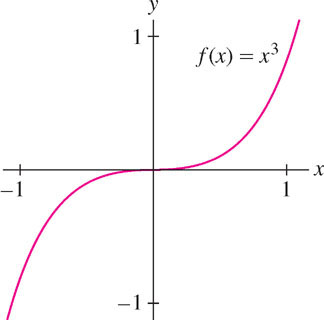
Fermat’s Theorem does not claim that all critical points yield local extrema. “False positives” may exist—that is, we might have \(f'(c) = 0\) without \(f(c)\) being a local min or max. For example, \(f(x) = x^{3}\) has derivative \(f'(x) = 3x^{2}\) and \(f'(0) = 0\), but \(f(0)\) is neither a local min nor max (Figure 4.15). The origin is a point of inflection (studied in Section 4.4), where the tangent line crosses the graph.
4.2.2 Optimizing on a Closed Interval
Finally, we have all the tools needed for optimizing a continuous function on a closed interval. Theorem 1 guarantees that the extreme values exist, and the next theorem tells us where to find them, namely among the critical points or endpoints of the interval.
In this section, we restrict our attention to closed intervals because in this case extreme values are guaranteed to exist (Theorem 1). Optimization on open intervals is discussed in Section 4.7.
THEOREM 3 Extreme Values on a Closed Interval
Assume that \(f(x)\) is continuous on \([a, b]\) and let \(f(c)\) be the minimum or maximum value on \([a, b]\). Then \(c\) is either a critical point or one of the endpoints \(a\) or \(b\).
Proof
If \(c\) is one of the endpoints \(a\) or \(b\), there is nothing to prove. If not, then \(c\) belongs to the open interval \((a, b)\). In this case, \(f(c)\) is also a local min or max because it is the min or max on \((a, b)\). By Fermat’s Theorem, \(c\) is a critical point.
EXAMPLE 3
Find the extrema of \(f(x) = 2x^{3} - 15x^{2} + 24x + 7\) on \([0, 6]\).
Solution The extreme values occur at critical points or endpoints by Theorem 3, so we can break up the problem neatly into two steps.
219
Step 1. Find the critical points.
The function \(f(x)\) is differentiable, so we find the critical points by solving
\[f'(x) = 6x^{2} -30x + 24 = 6(x - 1)(x - 4) = 0\]
The critical points are \(c = 1\) and \(4\).
Step 2. Compare values at the critical points and endpoints.
The maximum of \(f(x)\) on \([0, 6]\) is the largest of the values in this table, namely \(f(6) = 43\). Similarly, the minimum is \(f(4) = -9\). See Figure 4.16.
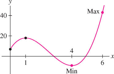
| \(x\)-value | Value of \(f\) |
|---|---|
| \(1\) (critical point) | \(f(1)=18\) |
| \(4\) (critical point) | \(f(4)=-9\) min |
| \(0\) (endpoint) | \(f(0)=7\) |
| \(6\) (endpoint) | \(f(6)=43\) max |
EXAMPLE 4 Function with a Cusp
Find the max of \(f(x) = 1 - (x - 1)^{\frac{2}{3}}\) on \([-1, 2]\).
Solution First, find the critical points:
\[ f'(x) = -\frac{2}{3} (x - 1)^{-\frac{1}{3}} = -\frac{2}{3(x-1)^{1/3}} \]
The equation \(f'(x) = 0\) has no solutions because \(f'(x)\) is never zero. However, \(f'(x)\) does not exist at \(x = 1\), so \(c = 1\) is a critical point (Figure 4.17).
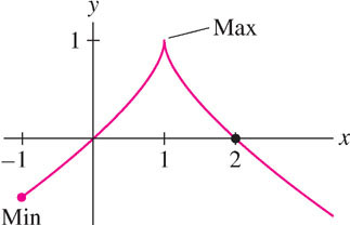
| \(x\)-value | Value of \(f\) |
|---|---|
| \(1\) (critical point) | \(f(1) = 1\) max |
| \(-1\) (endpoint) | \(f(-1)\approx-0.59\) min |
| \(2\) (endpoint) | \(f(2)=0\) |
Next, compare values at the critical points and endpoints.
Question 4.4 Extrema Progress Check 2
Find the absolute extrema of \(\displaystyle f(x)= |x|e^x\) on the interval \([-1,1]\).
| A. |
| B. |
| C. |
| D. |
EXAMPLE 5 Logarithmic Example
Find the extreme values of the function \(f(x) = x^{2} - 8 \ln x\) on \([1, 4]\).
Solution First, solve for the critical points:
\[ f'(x) = 2x - \frac{8}{x} = 0 \implies 2x = \frac{8}{x} \implies x=\pm 2 \]
The only critical point in the interval \([1, 4]\) is \(c = 2\). Next, compare the values of \(f(x)\) at the critical points and endpoints (Figure 4.18):
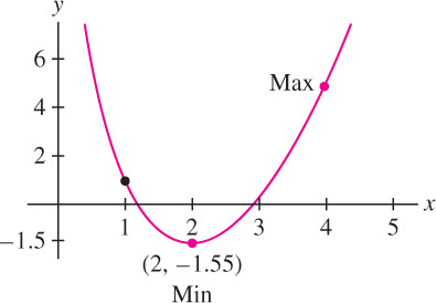
| \(x\)-value | Value of \(f\) |
|---|---|
| \(2\) (critical point) | \(f(2)\approx -1.55\) min |
| \(1\) (endpoint) | \(f(1)= 1\) |
| \(2\) (endpoint) | \(f(4)\approx4.9\) max |
We see that the min on \([1, 4]\) is \(f(2) \approx -1.55\) and the max is \(f(4) \approx 4.9\).
220
EXAMPLE 6 Trigonometric Function
Find the min and max of the function \(f(x) = \sin x + \cos^{2}x\) on \([0, 2\pi ]\) (Figure 4.19).
Solution First, solve for the critical points:
\begin{gather*} f'(x) = \cos x -2 \sin x\cos x = \cos x(1-2\sin x)=0\implies \cos x = 0 \text{ or }\sin x = \frac{1}{2}\\ \cos x = 0\implies x = \frac{\pi}{2},\frac{3\pi}{2}\text{ and }\sin x=\frac{1}{2}\implies x=\frac{\pi}{6},\frac{5\pi}{6} \end{gather*}
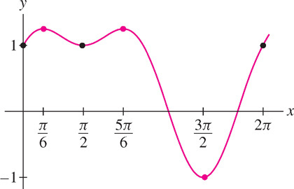
Then compare the values of \(f(x)\) at the critical points and endpoints: \[\begin{array}{llc} \hline x\text{-value}&\text{Value of }f&\\ \hline \tfrac{\pi}{2}\text{ (critical point)}&f\left(\tfrac{\pi}{2}\right) = 1+0^2 = 1&\\ \tfrac{3\pi}{2}\text{ (critical point)}&f\left(\tfrac{3\pi}{2}\right) = -1+0^2 = -1&\text{min}\\ \tfrac{\pi}{6}\text{ (critical point)}&f\left(\tfrac{\pi}{6}\right) = \tfrac{1}{2}+\left(\tfrac{\sqrt{3}}{2}\right)^2 = \tfrac{5}{4}&\text{max}\\ \tfrac{5\pi}{6}\text{ (critical point)}&f\left(\tfrac{5\pi}{6}\right) = \tfrac{1}{2}+\left(-\tfrac{\sqrt{3}}{2}\right)^2 = \tfrac{5}{4}&\text{max}\\ 0\text{ and }2\pi\text{ (endpoints)}&f(0)=f(2\pi)=1&\\ \hline \end{array}\]
Question 4.5 Extrema Progress Check 3
Find the absolute extrema of \(\displaystyle f(x)= -2x^3+15x^2-36x+27\) on the interval \([1,4]\).
| A. |
| B. |
| C. |
| D. |
4.2.3 Rolle’s Theorem
As an application of our optimization methods, we prove Rolle’s Theorem: If \(f(x)\) takes on the same value at two different points \(a\) and \(b\), and \(f(x)\) is differentiable between \(a\) and \(b\), and continuous on \([a,b]\), then somewhere between these two points the derivative is zero. Graphically: If the secant line between \(x = a\) and \(x = b\) is horizontal, then at least one tangent line between \(a\) and \(b\) is also horizontal (Figure 4.20).
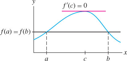
THEOREM 4 Rolle’s Theorem
Assume that \(f(x)\) is continuous on \([a, b]\) and differentiable on \((a, b)\). If \(f(a) = f(b)\), then there exists a number \(c\) between \(a\) and \(b\) such that \(f'(c) = 0\).
Proof
Since \(f(x)\) is continuous and \([a, b]\) is closed, \(f(x)\) has a min and a max in \([a, b]\). Where do they occur? If either the min or the max occurs at a point \(c\) in the open interval \((a, b)\), then \(f(c)\) is a local extreme value and \(f'(c) = 0\) by Fermat’s Theorem (Theorem 2). Otherwise, both the min and the max occur at the endpoints. However, \(f(a) = f(b)\), so in this case, the min and max coincide and \(f(x)\) is a constant function with zero derivative. Therefore, \(f'(c) = 0\) for all \(c \in (a, b)\).
EXAMPLE 7 Illustrating Rolle’s Theorem
Verify Rolle’s Theorem for
\[ f(x) = x^4 - x^2 \qquad\text{on }[-2,2] \]
Solution The hypotheses of Rolle’s Theorem are satisfied because \(f(x)\) is differentiable (and therefore continuous) everywhere, and \(f(2) = f(-2)\):
\[f(2) = 2^4 - 2^2 = 12\quad f(-2)=(-2)^4 - (-2)^2 = 12\]
We must verify that \(f'(c) = 0\) has a solution in \((-2, 2)\), so we solve \(f'(x) = 4x^{3} - 2x = 2x(2x^{2} - 1) = 0\). The solutions are \(c = 0\) and \(c=\pm\frac{1}{\sqrt{2}}\approx\pm0.707\). They all lie in \((-2, 2)\), so Rolle’s Theorem is satisfied with three values of \(c\).
EXAMPLE 8 Using Rolle’s Theorem
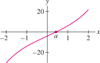
Show that \(f(x) = x^{3} + 9x - 4\) has precisely one real root.
221
Solution First, we note that \(f(0) = -4\) is negative and \(f(1) = 6\) is positive. By the Intermediate Value Theorem (Section 2.8), \(f(x)\) has at least one root \(a\) in \([0, 1]\). If \(f(x)\) had a second root \(b\), then \(f(a) = f(b) = 0\) and Rolle’s Theorem would imply that \(f'(c) = 0\) for some \(c \in (a, b)\). This is not possible because \(f'(x) = 3x^{2} + 9 \geq 9\), so \(f'(c) = 0\) has no solutions. We conclude that \(a\) is the only real root of \(f(x)\) (Figure 4.21).
We can hardly expect a more general method… This method never fails and could be extended to a number of beautiful problems; with its aid we have found the centers of gravity of figures bounded by straight lines or curves, as well as those of solids, and a number of other results which we may treat elsewhere if we have the time to do so.
—From Fermat’s On Maxima and Minima and on Tangents
HISTORICAL PERSPECTIVE
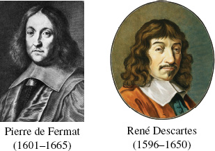
Sometime in the 1630’s, in the decade before Isaac Newton was born, the French mathematician Pierre de Fermat invented a general method for finding extreme values. Fermat said, in essence, that if you want to find extrema, you must set the derivative equal to zero and solve for the critical points, just as we have done in this section. He also described a general method for finding tangent lines that is not essentially different from our method of derivatives. For this reason, Fermat is often regarded as an inventor of calculus, together with Newton and Leibniz.
At around the same time, René Descartes (1596-1650) developed a different but less effective approach to finding tangent lines. Descartes, after whom Cartesian coordinates are named, was a profound thinker—the leading philosopher and scientist of his time in Europe. He is regarded today as the father of modern philosophy and the founder (along with Fermat) of analytic geometry. A dispute developed when Descartes learned through an intermediary that Fermat had criticized his work on optics. Sensitive and stubborn, Descartes retaliated by attacking Fermat’s method of finding tangents and only after some third-party refereeing did he admit that Fermat was correct. He wrote:
…Seeing the last method that you use for finding tangents to curved lines, I can reply to it in no other way than to say that it is very good and that, if you had explained it in this manner at the outset, I would have not contradicted it at all.
However, in subsequent private correspondence, Descartes was less generous, referring at one point to some of Fermat’s work as “le galimatias le plus ridicule”—the most ridiculous gibberish. Today Fermat is recognized as one of the greatest mathematicians of his age who made far-reaching contributions in several areas of mathematics.
4.2.4 Section 4.2 Summary
- The extreme values of \(f(x)\) on an interval \(I\) are the minimum and maximum values of \(f(x)\) for \(x \in I\) (also called absolute extrema on \(I\)).
- Basic Theorem: If \(f(x)\) is continuous on a closed interval \([a, b]\), then \(f(x)\) has both a min and a max on \([a, b]\).
- \(f(c)\) is a local minimum if \(f(x) \geq f(c)\) for all \(x\) in some open interval around \(c\). Local maxima are defined similarly.
- \(x = c\) is a critical point of \(f(x)\) if either \(f'(c) = 0\) or \(f'(c)\) does not exist.
- Fermat’s Theorem: If \(f(c)\) is a local min or max, then \(c\) is a critical point.
- To find the extreme values of a continuous function \(f(x)\) on a closed interval \([a, b]\):
Step 1. Find the critical points of \(f(x)\) in \([a, b]\).
Step 2. Calculate \(f(x)\) at the critical points in \([a, b]\) and at the endpoints.
The min and max on \([a, b]\) are the smallest and largest among the values computed in Step 2.
- Rolle’s Theorem: If \(f(x)\) is continuous on \([a, b]\) and differentiable on \((a, b)\), and if \(f(a) = f(b)\), then there exists \(c\) between \(a\) and \(b\) such that \(f'(c) = 0\).
222