5.2 The Definite Integral
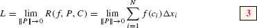
In the previous section, we saw that if f(x) is continuous on an interval [a, b], then the endpoint and midpoint approximations approach a common limit L as N → ∞:

300
When f(x) ≥ 0, L is the area under the graph of f(x). In a moment, we will state formally that L is the definite integral of f(x) over [a, b]. Before doing so, we introduce more general approximations called Riemann sums.
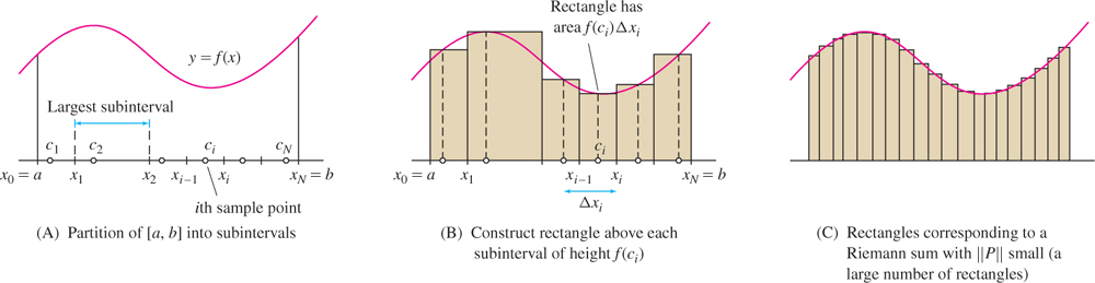
Recall that RN, LN, and MN use rectangles of equal width Δx, whose heights are the values of f(x) at the endpoints or midpoints of the subintervals. In Riemann sum approximations, we relax these requirements: The rectangles need not have equal width, and the height may be any value of f(x) within the subinterval.
To specify a Riemann sum, we choose a partition and a set of sample points:
- Partition P of size N: a choice of points that divides [a, b] into N subintervals.
P : a = x0 < x1 < x2 <⋯< xN = b
- Sample points C = {c1,…, cN}: ci belongs to the subinterval [xi−1, xi] for all i.
See Figures 1 and 2(A). The length of the ith subinterval [x[em]i[/em]−1, xi] is
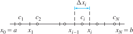
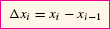
The norm of P, denoted ‖P‖, is the maximum of the lengths Δxi.
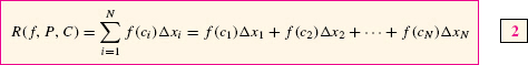
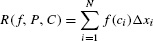
Given P and C, we construct the rectangle of height f(ci) and base Δxi over each subinterval [x[em]i[/em]−1, xi], as in Figure 2(B). This rectangle has area f(ci)Δxi if f(ci) ≥ 0. If f(ci) < 0, the rectangle extends below the x-axis, and f(ci)Δxi is the negative of its area. The Riemann sum is the sum
Keep in mind that RN, LN, and MN are particular examples of Riemann sums in which Δxi = (b − a)/N for all i, and the sample points ci are endpoints or midpoints.
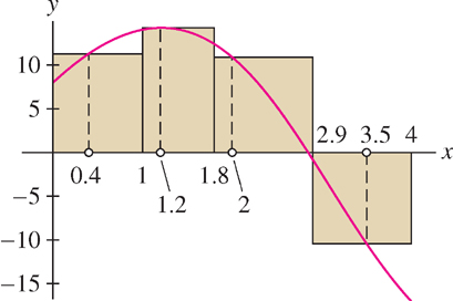
EXAMPLE 1
Calculate R(f, P, C), where f(x) = 8 + 12 sin x − 4x on [0, 4],
P : x0 = 0 < x1 = 1 < x2 = 1.8 < x3 = 2.9 < x4 = 4
C = {0.4, 1.2, 2, 3.5}
What is the norm ‖P‖?
Solution The widths of the subintervals in the partition (Figure 3) are

301
The norm of the partition is ‖P‖ = 1.1 since the two longest subintervals have width 1.1. Using a calculator, we obtain

Note in Figure 2(C) that as the norm ‖P‖ tends to zero (meaning that the rectangles get thinner), the number of rectangles N tends to ∞ and they approximate the area under the graph more closely. This leads to the following definition: f(x) is integrable over [a, b] if all of the Riemann sums (not just the endpoint and midpoint approximations) approach one and the same limit L as ‖P‖ tends to zero. Formally, we write
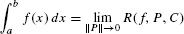
if |R(f, P, C) − L| gets arbitrarily small as the norm ‖P‖ tends to zero, no matter how we choose the partition and sample points. The limit L is called the definite integral of f(x) over [a, b].
DEFINITION Definite Integral
The definite integral of f(x) over [a, b], denoted by the integral sign, is the limit of Riemann sums:
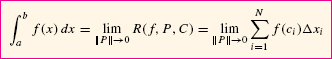
When this limit exists, we say that f(x) is integrable over [a, b].
The notation ∫ f(x)dx was introduced by Leibniz in 1686. The symbol ∫ is an elongated S standing for “summation.” The differential dx corresponds to the length Δxi along the x-axis.
The definite integral is often called, more simply, the integral of f(x) over [a, b]. The process of computing integrals is called integration. The function f(x) is called the integrand. The endpoints a and b of [a, b] are called the limits of integration. Finally, we remark that any variable may be used as a variable of integration (this is a “dummy” variable). Thus, the following three integrals all denote the same quantity:
One of the greatest mathematicians of the nineteenth century and perhaps second only to his teacher C. F. Gauss, Riemann transformed the fields of geometry, analysis, and number theory. Albert Einstein based his General Theory of Relativity on Riemann’s geometry. The “Riemann hypothesis” dealing with prime numbers is one of the great unsolved problems in present-day mathematics. The Clay Foundation has offered a $1 million prize for its solution (https://www.claymath.org/millennium).
CONCEPTUAL INSIGHT
Keep in mind that a Riemann sum R(f, P, C) is nothing more than an approximation to area based on rectangles, and that  is the number we obtain in the limit as we take thinner and thinner rectangles.
However, general Riemann sums (with arbitrary partitions and sample points) are rarely used for computations. In practice, we use particular approximations such as MN, or the Fundamental Theorem of Calculus, as we’ll learn in the next section. If so, why bother introducing Riemann sums? The answer is that Riemann sums play a theoretical rather than a computational role. They are useful in proofs and for dealing rigorously with certain discontinuous functions. In later sections, Riemann sums are used to show that volumes and other quantities can be expressed as definite integrals.

The next theorem assures us that continuous functions (and even functions with finitely many jump discontinuities) are integrable (see Appendix D for a proof). In practice, we rely on this theorem rather than attempting to prove directly that a given function is integrable.
302
THEOREM 1
If f(x) is continuous on [a, b], or if f(x) is continuous with at most finitely many jump discontinuities, then f(x) is integrable over [a, b].
Interpretation of the Definite Integral as Signed Area
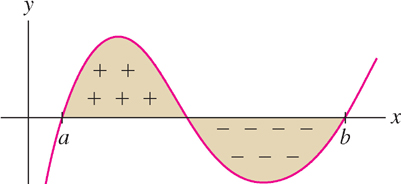
When f(x) ≥ 0, the definite integral defines the area under the graph. To interpret the integral when f(x) takes on both positive and negative values, we define the notion of signed area, where regions below the x-axis are considered to have “negative area” (Figure 4); that is,

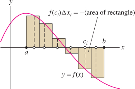
Now observe that a Riemann sum is equal to the signed area of the corresponding rectangles:
R(f, C, P) = f(c1)Δx1 + f(c2)Δx2 +⋯+ f(cN)ΔxN
Indeed, if f(ci) < 0, then the corresponding rectangle lies below the x-axis and has signed area f(ci)Δxi (Figure 5). The limit of the Riemann sums is the signed area of the region between the graph and the x-axis:
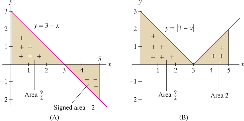
EXAMPLE 2 Signed Area
Calculate
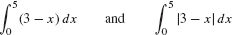
Solution The region between y = 3 − x and the x-axis consists of two triangles of areas  and 2 [Figure 6(A)]. However, the second triangle lies below the x-axis, so it has signed area −2. In the graph of y = |3 − x|, both triangles lie above the x-axis [Figure 6(B)]. Therefore,

303
Properties of the Definite Integral
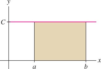
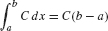
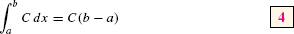
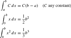
In the rest of this section, we discuss some basic properties of definite integrals. First, we note that the integral of a constant function f(x) = C over [a, b] is the signed area C(b − a) of a rectangle (Figure 7).
 .
.
THEOREM 2 Integral of a Constant
Next, we state the linearity properties of the definite integral.
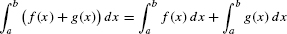
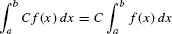
THEOREM 3 Linearity of the Definite Integral
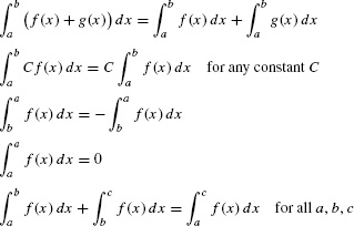
If f and g are integrable over [a, b], then f + g and Cf are integrable (for any constant C), and
Proof
These properties follow from the corresponding linearity properties of sums and limits. For example, Riemann sums are additive:
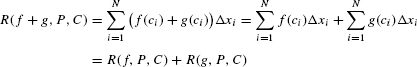
By the additivity of limits,
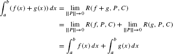
The second property is proved similarly.
EXAMPLE 3
Calculate  using the formula
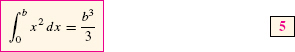
Solution
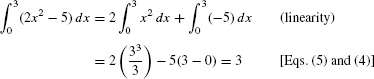
Eq. (5) was verified in Example 5 of Section 5.1.
304
So far we have used the notation  with the understanding that a < b. It is convenient to define the definite integral for arbitrary a and b.
DEFINITION Reversing the Limits of Integration
For a < b, we set
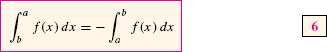
According to Eq. (6), the integral changes sign when the limits of integration are reversed. Since we are free to define symbols as we please, why have we chosen to put the minus sign in Eq. (6)? Because it is only with this definition that the Fundamental Theorem of Calculus holds true.
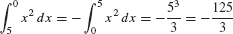
For example, by Eq. (5),
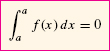
When a = b, the interval [a, b] = [a, a] has length zero and we define the definite integral to be zero:
EXAMPLE 4
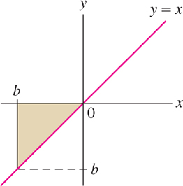
Prove that, for all b (positive or negative),
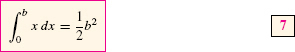
Solution If b > 0,  is the area
  of a triangle of base b and height b. If b < 0,
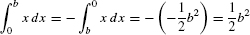
  is the signed area
  of the triangle in Figure 8, and Eq. (7) follows from the rule for reversing limits of integration:

Definite integrals satisfy an important additivity property: If f(x) is integrable and a ≤ b ≤ c as in Figure 9, then the integral from a to c is equal to the integral from a to b plus the integral from b to c. We state this in the next theorem (a formal proof can be given using Riemann sums).
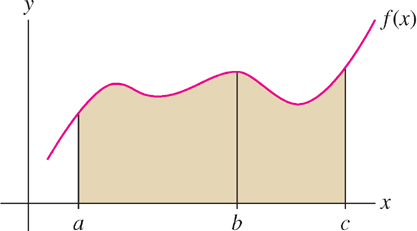
THEOREM 4 Additivity for Adjacent Intervals
Let a ≤ b ≤ c, and assume that f(x) is integrable. Then
This theorem remains true as stated even if the condition a ≤ b ≤ c is not satisfied (Exercise 88).
EXAMPLE 5
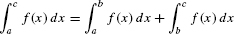
Calculate  .
.
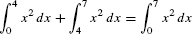
Solution Before we can apply the formula  from Example 3, we must use the additivity property for adjacent intervals to write
305
Now we can compute our integral as a difference:
Another basic property of the definite integral is that larger functions have larger integrals (Figure 10).
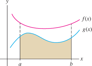
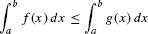
THEOREM 5 Comparison Theorem
If f and g are integrable and g(x) ≤ f(x) for x in [a, b], then
Proof
If g(x) ≤ f(x), then for any partition and choice of sample points, we have g(ci)Δxi ≤ f(ci)Δxi for all i. Therefore, the Riemann sums satisfy
Taking the limit as the norm ‖P‖ tends to zero, we obtain
EXAMPLE 6
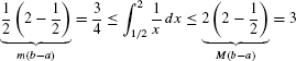
Prove the inequality: 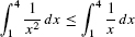 .
.
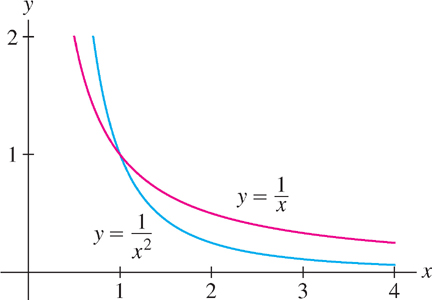
Solution If x ≥ 1, then x2 ≥ x, and x−2 ≤ x−1 [Figure 11]. Therefore, the inequality follows from the Comparison Theorem, applied with g(x) = x−2 and f(x) = x−1.
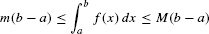
Suppose there are numbers m and M such that m ≤ f(x) ≤ M for x in [a, b]. We call m and M lower and upper bounds for f(x) on [a, b]. By the Comparison Theorem,
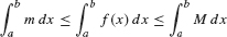
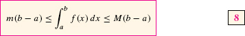
This says simply that the integral of f(x) lies between the areas of two rectangles (Figure 12).
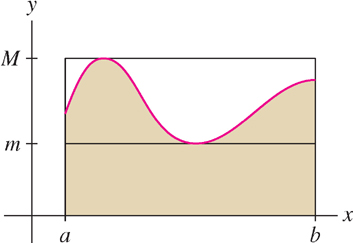
 dx lies between the areas of the rectangles of heights m and M.
EXAMPLE 7
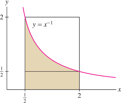
Prove the inequalities: 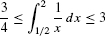 .
.
Solution Because f(x) = x−1 is decreasing (Figure 13), its minimum value on  is
is  and its maximum value is
  . By Eq. (8),
306
5.2.1 Summary
- A Riemann sum R(f, P, C) for the interval [a, b] is defined by choosing a partition
P : a = x0 < x1 < x2 <⋯< xN = b
and sample points C = {ci}, where ci ∈ [xi-1,xi]. Let Δxi = xi − x[em]i[/em]−1. Then
- The maximum of the widths Δxi is called the norm ‖P‖ of the partition.
- The definite integral is the limit of the Riemann sums (if it exists):
We say that f(x) is integrable over [a, b] if the limit exists.
- Theorem: If f(x) is continuous on [a, b], then f(x) is integrable over [a, b].
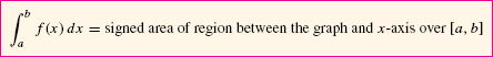
 = signed area of the region between the graph of f(x) and the x-axis.
- Properties of definite integrals:
- Formulas:
- Comparison Theorem: If f(x) ≤ g(x) on [a, b], then
If m ≤ f(x) ≤ M on [a, b], then
307