THE INTEGRAL

5.4 The Fundamental Theorem of Calculus, Part II

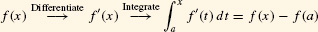
Part I of the Fundamental Theorem says that we can use antiderivatives to compute definite integrals. Part II turns this relationship around: It tells us that we can use the definite integral to construct antiderivatives.

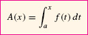
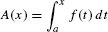
To state Part II, we introduce the area function of f with lower limit a:

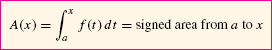
A(x) is sometimes called the cumulative area function. In the definition of A(x), we use t as the variable of integration to avoid confusion with x, which is the upper limit of integration. In fact, t is a dummy variable and may be replaced by any other variable.

In essence, we turn the definite integral into a function by treating the upper limit x as a variable (Figure 1). Note that A(a) = 0 because .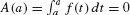

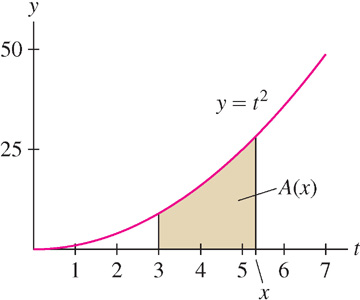
In some cases we can find an explicit formula for A(x) [Figure 2].

Figure 5.35: A(x) is the area under the graph from a to x.

Figure 5.36: The area under y = t² from 3 to x is

EXAMPLE 1

Find a formula for the area function .

Solution The function is an antiderivative for f(t) = t². By FTC I,

Note, in the previous example, that the derivative of A(x) is f(x) itself:

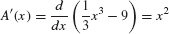
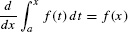
FTC II states that this relation always holds: The derivative of the area function is equal to the original function.

THEOREM 1 Fundamental Theorem of Calculus, Part II

Assume that f(x) is continuous on an open interval I and let a ∈ I. Then the area function

is an antiderivative of f(x) on I; that is, A′ (x) = f(x). Equivalently,

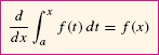
Furthermore, A(x) satisfies the initial condition A(a) = 0.

317

Proof

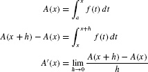
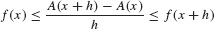
First, we use the additivity property of the definite integral to write the change in A(x) over [x, x + h] as an integral:

In other words, A(x + h) −A(x) is equal to the area of the thin sliver between the graph and the x-axis from x to x + h in Figure 3.

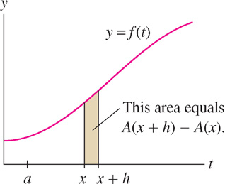
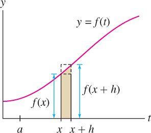
Figure 5.37: The area of the thin sliver equals A(x + h) −A(x).

Figure 5.38: The shaded sliver lies between the rectangles of heights f(x) and f(x + h).

To simplify the rest of the proof, we assume that f(x) is increasing (see Exercise 50 for the general case). Then, if h > 0, this thin sliver lies between the two rectangles of heights f(x) and f(x + h) in Figure 4, and we have

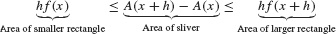
In this proof,

Now divide by h to squeeze the difference quotient between f(x) and f(x + h):

We have 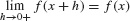because f(x) is continuous, and , so the Squeeze Theorem gives us

A similar argument shows that for h < 0,

Again, the Squeeze Theorem gives us

Equations (1) and (2) show that A′(x) exists and A′(x) = f(x).

CONCEPTUAL INSIGHT

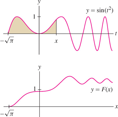
Many applications (in the sciences, engineering, and statistics) involve functions for which there is no explicit formula. Often, however, these functions can be expressed as definite integrals (or as infinite series). This enables us to compute their values numerically and create plots using a computer algebra system. Figure 5 shows a computer-generated graph of an antiderivative of f(x) = sin(x²), for which there is no explicit formula.

Figure 5.39: Computer-generated graph of

318

EXAMPLE 2 Antiderivative as an Integral

Let F(x) be the particular antiderivative of f(x) = sin (x²) satisfying . Express f(x) as an integral.

Solution According to FTC II, the area function with lower limit is an anti-derivative satisfying :

EXAMPLE 3 Differentiating an Integral

Find the derivative of

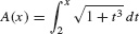
and calculate A′(2), A′(3), and A(2).

Solution By FTC II, . In particular,

On the other hand, .

CONCEPTUAL INSIGHT

The FTC shows that integration and differentiation are inverse operations. By FTC II, if you start with a continuous function f(x) and form the integral , then you get back the original function by differentiating:

On the other hand, by FTC I, if you differentiate first and then integrate, you also recover f(x) [but only up to a constant f(a)]:

When the upper limit of the integral is a function of x rather than x itself, we use FTC II together with the Chain Rule to differentiate the integral.

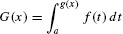
EXAMPLE 4 The FTC and the Chain Rule

Find the derivative of

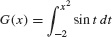
Solution FTC II does not apply directly because the upper limit is x² rather than x. It is necessary to recognize that G(x) is a composite function with outer function :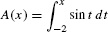

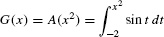
FTC II tells us that A′(x) = sin x, so by the Chain Rule,

G′(x) = A′(x²) · (x²)′ = sin(x²) · (2x) = 2x sin(x²)

Alternatively, we may set u = x² and use the Chain Rule as follows:

319

GRAPHICAL INSIGHT: Another Tale of Two Graphs

FTC II tells us that A′(x) = f(x), or, in other words, f(x) is the rate of change of A(x). If we did not know this result, we might come to suspect it by comparing the graphs of A(x) and f(x). Consider the following:

Figure 6 shows that the increase in area ΔA for a given Δx is larger at x₂ than at x₁ because f(x₂) > f(x₁). So the size of f(x) determines how quickly A(x) changes, as we would expect if A′(x) = f(x).

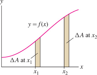Figure 5.40: The change in area ΔA for a given Δx is larger when f(x) is larger.
Figure 7 shows that the sign of f(x) determines whether A(x) is increasing or decreasing. If f(x) > 0, then A(x) is increasing because positive area is added as we move to the right. When f(x) turns negative, A(x) begins to decrease because we start adding negative area.

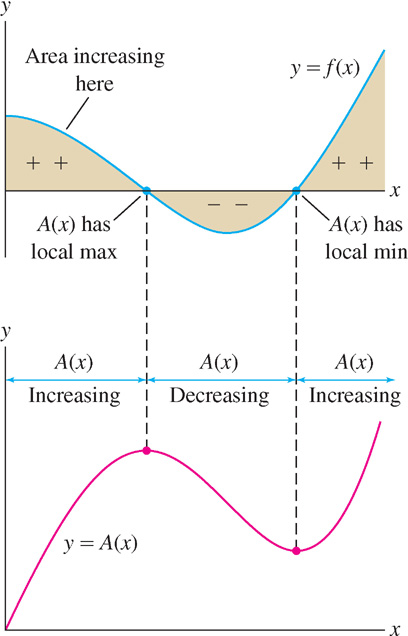Figure 5.41: The sign of f(x) determines the increasing/decreasing behavior of A(x).
A(x) has a local max at points where f(x) changes sign from + to − (the points where the area turns negative), and has a local min when f(x) changes from − to +. This agrees with the First Derivative Test.

These observations show that f(x) “behaves” like A′(x), as claimed by FTC II.

5.4.1 Summary

The area function with lower limit a: . It satisfies A(a) = 0.
FTC II: A′(x) = f(x), or, equivalently, .
FTC II shows that every continuous function has an antiderivative—namely, its area function (with any lower limit).
To differentiate the function , write G(x) = A(g(x)), where 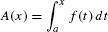. Then use the Chain Rule:
G′(x) = A′(g(x))g′(x) = f(g(x))g′(x)