5.5 Net Change as the Integral of a Rate
So far we have focused on the area interpretation of the integral. In this section, we use the integral to compute net change.
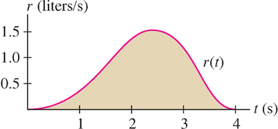
Consider the following problem: Water flows into an empty bucket at a rate of r(t) liters per second. How much water is in the bucket after 4 seconds? If the rate of water flow were constant—say, 1.5 liters/second—we would have
Quantity of water = flow rate × time elapsed = (1.5)4 = 6 liters
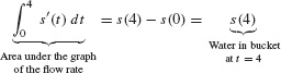
Suppose, however, that the flow rate r(t) varies as in Figure 5.42. Then the quantity of water is equal to the area under the graph of r(t). To prove this, let s(t) be the amount of water in the bucket at time t. Then s′(t) = r(t) because s′(t) is the rate at which the quantity of water is changing. Furthermore, s(0) = 0 because the bucket is initially empty. By FTC I,
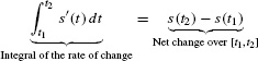
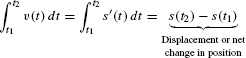
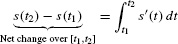
More generally, s(t2) − s(t1)is the net change in s(t) over the interval [t1, t2]. FTC I yields the following result.
THEOREM 1 Net Change as the Integral of a Rate
The net change in s(t) over an interval [t1, t2] is given by the integral
In Theorem 1, the variable t does not have to be a time variable.
323
EXAMPLE 1
Water leaks from a tank at a rate of 2 + 5t liters/hour, where t is the number of hours after 7 AM. How much water is lost between 9 and 11 AM?
Solution Let s(t) be the quantity of water in the tank at time t. Then s′(t) = −(2 + 5t), where the minus sign occurs because s(t) is decreasing. Since 9 AM and 11 AM correspond to t = 2 and t = 4, respectively, the net change in s(t) between 9 and 11 AM is
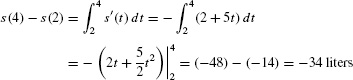
The tank lost 34 liters between 9 and 11 AM.
In the next example, we estimate an integral using numerical data. We shall compute the average of the left-and right-endpoint approximations, because this is usually more accurate than either endpoint approximation alone. (In Section 7.8, this average is called the Trapezoidal Approximation.)
EXAMPLE 2 Traffic Flow
The number of cars per hour passing an observation point along a highway is called the traffic flow rate q(t) (in cars per hour).
- (a) Which quantity is represented by the integral

- (b) The flow rate is recorded at 15-min intervals between 7:00 and 9:00 AM. Estimate the number of cars using the highway during this 2-hour period.
t 7:00 7:15 7:30 7:45 8:00 8:15 8:30 8:45 9:00 q(t) 1044 1297 1478 1844 1451 1378 1155 802 542
Solution
- (a) The integral
 represents the total number of cars that passed the observation point during the time interval [t1, t2].
 - (b) The data values are spaced at intervals of Δt = 0.25 hour. Thus,
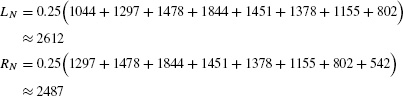
In Example 2, LN is the sum of the values of q(t) at the left endpoints
and RN is the sum of the values of q(t) at the right endpoints
We estimate the number of cars that passed the observation point between 7 and 9 AM by taking the average of RN and LN:
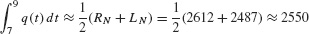
Approximately 2550 cars used the highway between 7 and 9 AM.
The Integral of Velocity
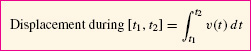
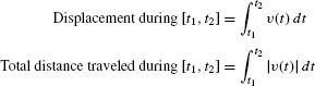
Let s(t) be the position at time t of an object in linear motion. Then the object’s velocity is v(t) = s′(t), and the integral of v(t) is equal to the net change in position or displacement over a time interval [t1, t2]:
324
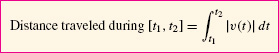
We must distinguish between displacement and distance traveled. If you travel 10 km and return to your starting point, your displacement is zero but your distance traveled is 20 km. To compute distance traveled rather than displacement, integrate the speed |v(t)|.
THEOREM 2 The Integral of Velocity
For an object in linear motion with velocity v(t), then
EXAMPLE 3
A particle has velocity v(t) = t3 −10t2 + 24t m/s. Compute:
- (a) Displacement over [0, 6]
- (b) Total distance traveled over [0, 6]
Indicate the particle’s trajectory with a motion diagram.
Solution First, we compute the indefinite integral:

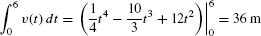
- (a) The displacement over the time interval [0, 6] is
- (b) The factorization v(t) = t(t − 4)(t − 6) shows that v(t) changes sign at t = 4. It is positive on [0, 4] and negative on [4, 6] as we see in Figure 5.43.
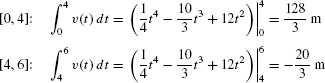
Therefore, the total distance traveled is
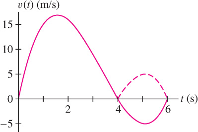 Figure 5.43: Graph of v(t) = t3 − 10t2 + 24t. Over [4, 6], the dashed curve is the graph of |v(t)|.
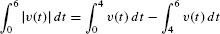
We evaluate these two integrals separately:
The total distance traveled is 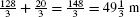
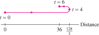
Figure 5.44 is a motion diagram indicating the particle’s trajectory. The particle travels  during the first 4 s and then backtracks
  over the next 2 s.
325
Total versus Marginal Cost
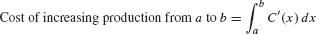
Consider the cost function C(x) of a manufacturer (the dollar cost of producing x units of a particular product or commodity). The derivative C′(x) is called the marginal cost. The cost of increasing production from a to b is the net change C(b) − C(a), which is equal to the integral of the marginal cost:
In Section 3.4, we defined the marginal cost at production level x0 as the cost
C(x0 + 1) − C(x0)
of producing one additional unit. Since this marginal cost is approximated well by the derivative C′(x0), we often refer to C′(x) itself as the marginal cost.
EXAMPLE 4
The marginal cost of producing x computer chips (in units of 1000) is C′(x) = 300x2 − 4000x + 40,000 (dollars per thousand chips).
- (a) Find the cost of increasing production from 10,000 to 15,000 chips.
- (b) Determine the total cost of producing 15,000 chips, assuming that it costs $30,000 to set up the manufacturing run [that is, C(0) = 30,000].
Solution
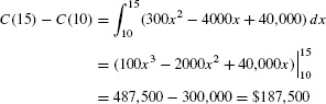
- (a) The cost of increasing production from 10,000 (x = 10) to 15,000 (x = 15) is
- (b) The cost of increasing production from 0 to 15,000 chips is
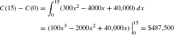
The total cost of producing 15,000 chips includes the set-up costs of $30,000:
C(15) = C(0) + 487,500 = 30,000 + 487,500 = $517,500
5.5.1 Summary
- Many applications are based on the following principle: The net change in a quantity s(t) is equal to the integral of its rate of change:
- For an object traveling in a straight line at velocity v(t),
- If C(x) is the cost of producing x units of a commodity, then C′(x) is the marginal cost and
Further Insights and Challenges
Question 5.18
Show that a particle, located at the origin at t = 1 and moving along the x-axis with velocity v(t) = t−2, will never pass the point x = 2.
Question 5.19
Show that a particle, located at the origin at t = 1 and moving along the x-axis with velocity v(t) = t−1/2 moves arbitrarily far from the origin after sufficient time has elapsed.