5.7 Further Transcendental Functions
Recall that
\[\boxed{\bbox[#FAF8ED,5pt]{\log_e x = \ln x := \int \limits_1^x \dfrac{dt}{t} \hskip 20pt \mbox{for} \ x>0}}\tag {1}\]
Thus, by FTC I,
\[ \int \limits_a^b \dfrac{dx}{x} = \ln \dfrac{b}{a} \]
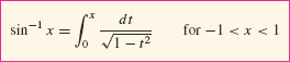
In a similar fashion, we can express \(\sin^{-1} x\) as a definite integral using the derivative formula from Section 3.9 (Figure 5.49):

Since sin−1 0 = 0, we have
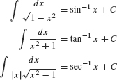
On the other hand, the derivative formulas from Section 3.8 yield integration formulas that are useful for evaluating new types of integrals.
Inverse Trigonometric Functions


It is possible (and mathematically, it is more efficient) to take Eq. (1) as the definition of ln x and to define ex as the corresponding inverse function (see Exercises 78–79).
337
In this list, we omit the integral formulas corresponding to the derivatives of cos−1x, cot−1x, and csc−1x because the integrals differ only by a minus sign from those already on the list. For example,

EXAMPLE 1
Evaluate  .
.
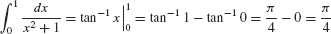
Solution This integral is the area of the region in Figure 5.50. By Eq. (3),
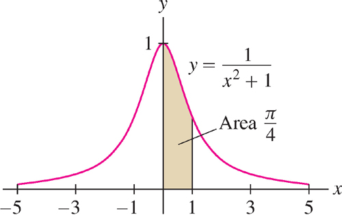
 .
.
EXAMPLE 2 Using Substitution
Evaluate 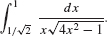
Solution Notice that  can be written as
  , so it makes sense to try the substitution u = 2x, du = 2 dx. Then

The new limits of integration are  . By Eq. (4),
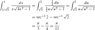
In substitution, we usually define u as a function of x. Sometimes, it is more convenient to define x as a function of u. We do this here, where we set x = 2u.
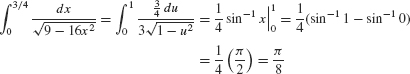
EXAMPLE 3 Using Substitution
Evaluate  .
.
Solution Let us first rewrite the integrand:
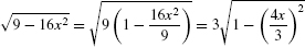
Thus it makes sense to use the substitution  . Then
  and
and

The new limits of integration are u (0) = 0 and  :
:
338
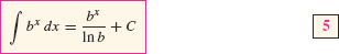
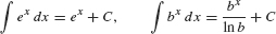
Integrals Involving \(f(x)=b^x\)
The exponential function f(x) = ex is particularly convenient because ex is both its own derivative and its own antiderivative. For other bases \(b>0\), we have

This translates into the integral formula
![]() REMINDER
\[b=e^{\ln b}, b^x=e^{(\ln b) x}\]
REMINDER
\[b=e^{\ln b}, b^x=e^{(\ln b) x}\]
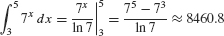
EXAMPLE 4
Evaluate  .
.
Solution Apply Eq. (5) with b = 7.
EXAMPLE 5
Evaluate 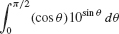 .
.
Solution Use the substitution u = sin θ, du = cos θ dθ. The new limits of integration become u (0) = 0 and u(π/2) = 1:

5.7.1 Summary
- Integral formula for the natural logarithm: \[\log_e x = \ln x := \int \limits_1^x \frac{dt}{t}\]
- Integral formulas:
- Integrals of exponential functions (b > 0, b ≠ 1):
339