6.2 Setting Up Integrals: Volume, Density, Average Value
Which quantities are represented by integrals? Roughly speaking, integrals represent quantities that are the “total amount” of something such as area, volume, or total mass. There is a two-step procedure for computing such quantities: (1) Approximate the quantity by a sum of \(N\) terms, and (2) Pass to the limit as \(N\to\infty\) to obtain an integral. We'll use this procedure often in this and other sections.
Volume
The term “solid” or “solid body” refers to a solid three-dimensional object.
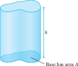
Our first example is the volume of a solid body. Before proceeding, let's recall that the volume of a right cylinder (Figure 6.8) is \(Ah\), where \(A\) is the area of the base and \(h\) is the height, measured perpendicular to the base. Here we use the “right cylinder” in the general sense; the base does not have to be circular, but the sides are perpendicular to the base.
Suppose that the solid body extends from height \(y=a\) to \(y=b\) along the \(y\)-axis as in Figure 6.9. Let \(A(y)\) be the area of the horizontal cross section at height \(y\) (the intersection of the solid with the horizontal plane at height \(y\)).
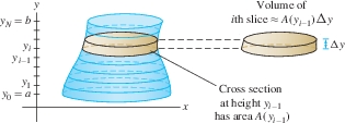
To compute the volume \(V\) of the body, divide the body into \(N\) horizontal slices of thickness \(\Delta y=({b-a})/{N}\). The \(i\)th slice extends from \(y_{i-1}\) to \(y_i\), where \(y_i = a + i\Delta y\). Let \(V_i\) be the volume of the slice.
If \(N\) is very large, then \(\Delta y\) is very small and the slices are very thin. In this case, the \(i\)th slice is nearly a right cylinder of base \(A(y_{i-1})\) and height \(\Delta y\), and therefore \(V_i\approx A(y_{i-1})\Delta y\). Summing up, we obtain \[ V =\sum_{i=1}^N V_i\approx \sum_{i=1}^N \, A(y_{i-1})\Delta y \] The sum on the right is a left-endpoint approximation to the integral \(\int_a^b A(y)\,\mathrm{d}y\). If we assume that \(A(y)\) is a continuous function, then the approximation improves in accuracy and converges to the integral as \(N\to\infty\). We conclude that the volume of the solid is equal to the integral of its cross-sectional area.
Volume as the Integral of Cross-Sectional Area
Let \(A(y)\) be the area of the horizontal cross section at height \(y\) of a solid body extending from \(y=a\) to \(y=b\). Then \[ \boxed{\bbox[#FAF8ED,5pt]{\displaystyle\textrm{Volume of the solid body}=\int\limits_a^b A(y)\, \mathrm{d}y }}\tag {1} \]
366
EXAMPLE 1 Volume of a Pyramid
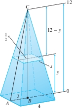
Calculate the volume \(V\) of a pyramid of height 12 m whose base is a square of side 4 m.
Solution To use Eq. (1), we need a formula for the horizontal cross section \(A(y)\).
Step 1. Find a formula for \(A(y)\)
Figure 6.10 shows that the horizontal cross section at height \(y\) is a square. To find the side \(s\) of this square, apply the law of similar triangles to \(\triangle ABC\) and to the triangle of height \(12-y\) whose base of length \(\frac{1}{2}s\) lies on the cross section: \[ \frac{\textrm{Base}}{\textrm{Height}} = \frac{2}{12} =\frac{\frac{1}{2}s}{12-y}\quad\Rightarrow\quad 2(12 - y) = 6s \]
We find that \(s =\frac13(12-y)\) and therefore \(A(y)=s^2=\frac19(12-y)^2\).
Step 2. Compute \(V\) as the integral of \(A(y)\)
\[ V = \int\limits_0^{12}\,A(y)\,\mathrm{d}y = \int\limits_0^{12}\frac19(12-y)^2\,\mathrm{d}y=-\frac1{27}(12-y)^3\Big|_0^{12}=64 \mathrm{m}^3 \] This agrees with the result obtained using the formula \(V=\frac13Ah\) for the volume of a pyramid of base \(A\) and height \(h\), since \(\frac13Ah=\frac13(4^2)(12)=64\).
Question 6.4 Cavalieri's Principle Progress Check Question 1
Calculate the volume \(V\) in cubic meters of a pyramid of height 15 m whose base is a square of side 3m. (Do not enter units)
EXAMPLE 2
Compute the volume \(V\) of the solid in Figure 6.11, whose base is the region between the inverted parabola \(y=4-x^2\) and the \(x\)-axis, and whose vertical cross sections perpendicular to the \(y\)-axis are semicircles.
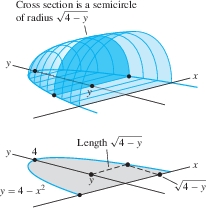
Solution To find a formula for the area \(A(y)\) of the cross section, observe that \(y=4-x^2\) can be written \(x=\pm\sqrt{4-y}\). We see in Figure 6.11 that the cross section at \(y\) is a semicircle of radius \(r=\sqrt{4-y}\). This semicircle has area \(A(y)= \frac12 \pi r^2= \frac{\pi}{2}(4-y)\). Therefore \[ V = \int\limits_0^4A(y)\,\mathrm{d}y = \frac{\pi}2\int\limits_0^4 (4-y)\,\mathrm{d}y = \frac{\pi}2 \left(4y-\frac12y^2\right)\bigg|_0^4 = 4\pi \]
In the next example, we compute volume using vertical rather than horizontal cross sections. This leads to an integral with respect to \(x\) rather than \(y\).
EXAMPLE 3 Volume of a Sphere: Vertical Cross Sections
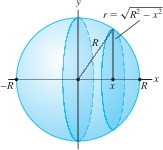
Compute the volume of a sphere of radius \(R\).
Solution As we see in Figure 6.12, the vertical cross section of the sphere at \(x\) is a circle whose radius \(r\) satisfies \(x^2+r^2=R^2\) or \(r=\sqrt{R^2 - x^2}\). The area of the cross section is \(A(x) = \pi r^2 = \pi(R^2 - x^2)\). Therefore, the sphere has volume \[ \int\limits_{-R}^R \pi(R^2 - x^2)\, \mathrm{d}x = \pi \left(R^2x - \frac{x^3}{3}\right)\bigg|_{-R}^R = 2 \left(\pi R^3 - \pi\frac{R^3}{3}\right) = \frac{4}{3}\pi R^3 \]
367
CONCEPTUAL INSIGHT
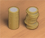
Cavalieri's principle states: Solids with equal cross-sectional areas have equal volume. It is often illustrated convincingly with two stacks of coins (Figure 6.13). Our formula \(V=\int^b_a A(y)\,\mathrm{d}y\) includes Cavalieri's principle, because the volumes \(V\) are certainly equal if the cross-sectional areas \(A(y)\) are equal.
Density
Next, we show that the total mass of an object can be expressed as the integral of its mass density. Consider a rod of length \(\ell\). The rod's linear mass density \(\rho\) is defined as the mass per unit length. If \(\rho\) is constant, then by definition, \[ \begin{equation} \textrm{Total~mass} = \textrm{linear mass density} \times \textrm{length} = \rho\cdot \ell \tag {2} \end{equation} \] For example, if \(\ell=10\) cm and \(\rho = 9 \mathrm{g\text{/}cm}\), then the total mass is \(\rho\ell=9\cdot 10=90\) g.
The symbol \(\rho\) (lowercase Greek letter rho) is used often to denote density.
Now consider a rod extending along the \(x\)-axis from \(x=a\) to \(x=b\) whose density \(\rho(x)\) is a continuous function of \(x\), as in Figure 6.14. To compute the total mass \(M\), we break up the rod into \(N\) small segments of length \(\Delta x = ({b-a})/{N}\). Then \(M=\sum_{i=1}^NM_i\), where \(M_i\) is the mass of the \(i\)th segment.
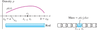
We cannot use Eq. (2) because \(\rho(x)\) is not constant, but we can argue that if \(\Delta x\) is small, then \(\rho(x)\) is nearly constant along the \(i\)th segment. If the \(i\)th segment extends from \(x_{i-1}\) to \(x_i\) and \(c_i\) is any sample point in \([x_{i-1},x_i]\), then \(M_i\approx \rho(c_i)\Delta x\) and \[ \textrm{Total mass}~M = \sum_{i=1}^N M_i \approx \sum_{i=1}^N\rho(c_i)\Delta x \] As \(N\to \infty\), the accuracy of the approximation improves. However, the sum on the right is a Riemann sum whose value approaches \({\int_a^b \rho(x)\, dx}\), and thus it makes sense to define the total mass of a rod as the integral of its linear mass density: \[ \begin{equation} \boxed{\bbox[#FAF8ED,5pt]{\textrm{Total mass} M = \int_a^b\, \rho(x)\, dx}} \tag {3} \end{equation} \]
Note the similarity in the way we use thin slices to compute volume and small pieces to compute total mass.
EXAMPLE 4 Total Mass
Find the total mass \(M\) of a 2-m rod of linear density \(\rho(x) = 1 + x(2-x) \mathrm{kg\text{/}m}\), where \(x\) is the distance from one end of the rod.
Solution
\[ \begin{align*} M = \int_0^2 \rho(x)\, dx = \int_0^2 \big(1+x(2-x)\big)\, dx = \left(x + x^2 - \frac{1}{3}x^3\right)\bigg|_0^2 = \frac{10}{3} \textrm{kg} \end{align*} \]
368
In some situations, density is a function of distance to the origin. For example, in the study of urban populations, it might be assumed that the population density \(\rho(r)\) (in people per square kilometer) depends only on the distance \(r\) from the center of a city. Such a density function is called a radial density function.
In general, density is a function \(\rho(x,y)\) that depends not just on the distance to the origin but also on the coordinates \((x,y)\). Total mass or population is then computed using double integration, a topic in multivariable calculus.
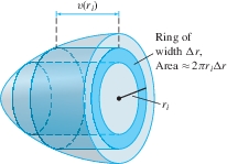
We now derive a formula for the total population \(P\) within a radius \(R\) of the city center assuming a radial density \(\rho(r)\). First, divide the circle of radius \(R\) into \(N\) thin rings of equal width \(\Delta r = R/N\) as in Figure 6.15.
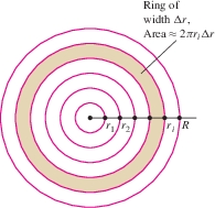
Let \(P_i\) be the population within the \(i\)th ring, so that \(P=\sum_{i=1}^N P_i\). If the outer radius of the \(i\)th ring is \(r_i\), then the circumference is \(2\pi r_i\), and if \(\Delta r\) is small, the area of this ring is approximately \(2\pi r_i\Delta r\) (outer circumference times width). Furthermore, the population density within the thin ring is nearly constant with value \(\rho(r_i)\). With these approximations, \[ \begin{array}{c} P_i \approx \underset{\hbox{Area of ring}}{\underbrace{2\pi r_i\Delta r}} \times \underset{\underset{\hbox{density}}{\hbox{Population}}}{\underbrace{\rho(r_i)}} = 2\pi r_i \rho(r_i)\Delta r \\ P = \sum_{i=1}^N P_i \approx 2\pi \sum_{i=1}^N r_i\rho(r_i)\Delta r \end{array} \] This last sum is a right-endpoint approximation to the integral \(2\pi \int_0^R r\rho(r)\, dr\). As \(N\) tends to \(\infty\), the approximation improves in accuracy and the sum converges to the integral. Thus, for a population with a radial density function \(\rho(r)\), \[ \begin{equation*} \boxed{\bbox[#FAF8ED,5pt]{\textrm{Population \(P\) within a radius \(R\)} = 2\pi \int_0^Rr\rho(r)\, dr }}\tag{4} \end{equation*} \]
Remember that for a radial density function, the total population is obtained by integrating \(2\pi r\rho (r)\) rather than \(\rho(r)\).
EXAMPLE 5 Computing Total Population
The population in a certain city has radial density function \(\rho(r) = 15(1+r^2)^{-1/2}\), where \(r\) is the distance from the city center in kilometers and \(\rho\) has units of thousands per square kilometer. How many people live in the ring between 10 and 30 km from the city center?
Solution The population \(P\) (in thousands) within the ring is \[ P = 2\pi \int_{10}^{30} r\big(15(1+r^2)^{-1/2}\big)\, dr = 2\pi(15) \int_{10}^{30} \frac{r}{(1+r^2)^{1/2}}\, dr \] Now use the substitution \(u=1+r^2\), \(du=2r\,dr\). The limits of integration become \(u(10)=101\) and \(u(30)=901\): \[ P = 30\pi \int_{101}^{901} u^{-1/2}\, \left(\frac12\right)du = 30\pi u^{1/2}\Big|_{101}^{901}\approx 1881 \textrm{thousand} \] In other words, the population is approximately 1.9 million people.
Flow Rate
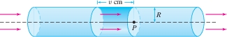
When fluid flows through a tube, the flow rate \(Q\) is the volume per unit time of fluid passing through the tube (Figure 6.16). The flow rate depends on the velocity of the fluid particles. If all particles of the fluid travel with the same velocity \(v\) (say, in units of cm\(^3\)/min), and the tube has radius \(R\), then \[ \underbrace{\textrm{Flow rate }Q}_{\textrm{Volume per unit time}} = \textrm{cross-sectional area} \times \textrm{velocity} =\pi R^2 v \mathrm{cm^3\text{/}min} \] Why is this formula true? Let's fix an observation point \(P\) in the tube and ask: Which fluid particles flow past \(P\) in a 1-min interval? A particle travels \(v\) centimeters each minute, so it flows past \(P\) during this minute if it is located not more than \(v\) centimeters to the left of \(P\) (assuming the fluid flows from left to right). Therefore, the column of fluid flowing past \(P\) in a 1-min interval is a cylinder of radius \(R\), length \(v\), and volume \(\pi R^2 v\) (Figure 6.16).
369
In reality, the fluid particles do not all travel at the same velocity because of friction. However, for a slowly moving fluid, the flow is laminar, by which we mean that the velocity \(v(r)\) depends only on the distance \(r\) from the center of the tube. The particles at the center of the tube travel most quickly, and the velocity tapers off to zero near the walls of the tube (Figure 6.17).
If the flow is laminar, we can express the flow rate \(Q\) as an integral. We divide the circular cross-section of the tube into \(N\) thin concentric rings of width \(\Delta r = R/N\) (Figure 6.18). The area of the \(i\)th ring is approximately \(2\pi r_i\Delta r\) and the fluid particles flowing past this ring have velocity that is nearly constant with value \(v(r_i)\). Therefore, we can approximate the flow rate \(Q_i\) through the \(i\)th ring by \[ Q_i \approx \textrm{cross-sectional area}\times\textrm{velocity} \approx (2\pi r_i\Delta r) v(r_i) \] We obtain \[ \smash{Q = \sum_{i=1}^N Q_i \approx 2\pi\sum_{i=1}^N r_i v(r_i)\Delta r} \] The sum on the right is a right-endpoint approximation to the integral \(2\pi\int_0^R rv(r)\, dr\). Once again, we let \(N\) tend to \(\infty\) to obtain the formula \[ \begin{equation} \boxed{\bbox[#FAF8ED,5pt]{\textrm{Flow rate } Q = 2\pi\int_0^R rv(r)\, dr}} \end{equation} \] Note the similarity of this formula and its derivation to that of population with a radial density function.
The French physician Jean Poiseuille (1799–1869) discovered the law of laminar flow that cardiologists use to study blood flow in humans. Poiseuille's Law highlights the danger of cholesterol buildup in blood vessels: The flow rate through a blood vessel of radius \(R\) is proportional to \(R^4\), so if \(R\) is reduced by one-half, the flow is reduced by a factor of 16.
EXAMPLE 6 Laminar Flow
According to Poiseuille's Law, the velocity of blood flowing in a blood vessel of radius \(R\) cm is \(v(r) = k(R^2 - r^2)\), where \(r\) is the distance from the center of the vessel (in centimeters) and \(k\) is a constant. Calculate the flow rate \(Q\) as function of \(R\), assuming that \(k= 0.5 (\hbox{cm-s})^{-1}\).
Solution By Eq. (5), \[ \begin{align*} Q &= 2\pi \int_0^R (0.5)r(R^2 - r^2)\, dr = \pi \left( R^2\frac{r^2}{2} - \frac{r^4}{4} \right) \bigg|_0^R = \frac{\pi}4\,R^4 \mathrm{cm^3\text{/}s} \end{align*} \] Note that \(Q\) is proportional to \(R^4\) (this is true for any value of \(k\)).
370
Average Value
As a final example, we discuss the average value of a function. Recall that the average of \(N\) numbers \(a_1, a_2, \ldots, a_N\) is the sum divided by \(N\): \[ \frac{a_1 + a_2 + \cdots + a_N}N = \frac{1}{N} \sum_{j=1}^N a_j \] For example, the average of 18, 25, 22, and 31 is \(\frac14(18+25+22+31) = 24\).
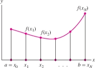
We cannot define the average value of a function \(f(x)\) on an interval \([a,b]\) as a sum because there are infinitely many values of \(x\) to consider. But recall the formula for the right-endpoint approximation \(R_N\) (Figure 6.19): \[ R_N = \frac{b-a}{N} \bigl(f(x_1) + f(x_2) + \cdots + f(x_N)\bigr) \] where \(x_i = a + i\left(\dfrac{b-a}{N}\right)\). We see that \(R_N\) divided by \((b-a)\) is equal to the average of the equally spaced function values \(f(x_i)\): \[ \frac{1}{b-a}\,R_N = \underbrace{\frac{f(x_1) + f(x_2) + \cdots + f(x_N)}{N}}_{\textrm{Average of the function values}} \] If \(N\) is large, it is reasonable to think of this quantity as an approximation to the average of \(f(x)\) on \([a,b]\). Therefore, we define the average value itself as the limit: \[ \textrm{Average value} = \lim_{N\to\infty} \frac{1}{b-a} R_N(f) = \frac{1}{b-a}\int_a^b f(x)\,dx \]
DEFINITION Average Value
The average value of an integrable function \(f(x)\) on \([a,b]\) is the quantity \[ \begin{equation*} \boxed{\bbox[#FAF8ED,5pt]{\textrm{Average value} = \frac{1}{b-a}\int_a^b f(x)\, dx}}\tag {6} \end{equation*} \]
The average value of a function is also called the mean value.
GRAPHICAL INSIGHT
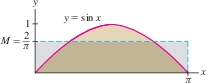
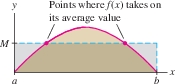
Think of the average value \(M\) of a function as the average height of its graph (Figure 6.20). The region under the graph has the same signed area as the rectangle of height \(M\), because \(\int_a^b\,f(x)\,dx = M(b-a)\).
EXAMPLE 7
Find the average value of \(f(x)=\sin x\) on \([0,\pi]\).
Solution The average value of \(\sin x\) on \([0,\pi]\) is \[ \frac{1}{\pi}\int_0^{\pi} \sin x\, dx = -\frac{1}{\pi}\cos x\bigg|_0^{\pi} = \frac{1}{\pi}\big({-(-1)} - (-1)\big) = \frac{2}{\pi} \approx 0.637 \] This answer is reasonable because \(\sin x\) varies from 0 to 1 on the interval \([0,\pi]\) and the average 0.637 lies somewhere between the two extremes (Figure 6.20).
371
EXAMPLE 8 Vertical Jump of a Bushbaby
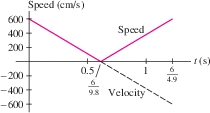
The bushbaby (Galago senegalensis) is a small primate with remarkable jumping ability (Figure 6.21). Find the average speed during a jump if the initial vertical velocity is \(v_0 = 600\) cm/s. Use Galileo's formula for the height \(h(t)=v_0t-\tfrac12 gt^2\) (in centimeters, where \(g=980 \textrm{ cm/s}^2\)).
Solution The bushbaby's height is \(h(t) = v_0 t - \frac12 gt^2 = t\big(v_0 - \frac{1}{2} gt\big)\). The height is zero at \(t=0\) and at \(t = {2v_0}/{g} = \frac{1200}{980} = \frac{6}{4.9}\) s, when jump ends.

The bushbaby's velocity is \(h'(t) = v_0 = gt = 600 - 980t\). The velocity is negative for \(t \gt {v_0}/{g} = \frac{6}{9.8}\), so as we see in Figure 6.22, the integral of speed \(|h'(t)|\) is equal to the sum of the areas of two triangles of base \(\frac{6}{9.8}\) and height 600: \[ \begin{align*} \int_0^{6/4.9}|600-980t|\,dt = \frac12\left(\frac{6}{9.8}\right)(600) + \frac12\left(\frac{6}{9.8}\right)(600) = \frac{3600}{9.8} \end{align*} \] The average speed \(\overline{s}\) is \[ \overline{s} = \frac1{\frac{6}{4.9}}\int_0^{6/4.9}|600-980t|\,dt = \frac1{\frac{6}{4.9}}\left(\frac{3600}{9.8}\right) = 300\,\,\textrm{cm/s} \]
There is an important difference between the average of a list of numbers and the average value of a continuous function. If the average score on an exam is 84, then 84 lies between the highest and lowest scores, but it is possible that no student received a score of 84. By contrast, the Mean Value Theorem (MVT) for Integrals asserts that a continuous function always takes on its average value somewhere in the interval (Figure 6.23).
For example, the average of \(f(x)=\sin x\) on \([0,\pi]\) is \(2/\pi\) by Example 7. We have \(f(c) = {2}/{\pi}\) for \(c =\sin^{-1}(2/\pi)\approx 0.69\). Since 0.69 lies in \([0,\pi]\), \(f(x)=\sin x\) indeed takes on its average value at a point in the interval.
THEOREM 1 Mean Value Theorem for Integrals
If \(f(x)\) is continuous on \([a,b]\), then there exists a value \(c\in[a,b]\) such that \[ f(c)=\frac{1}{b-a}\int_a^b f(x)\,dx \]
Proof
Let \(M=\frac1{b-a}\int_a^b\,f(x)\) be the average value. Because \(f(x)\) is continuous, we can apply Theorem 1 of Section 4.2 to conclude that \(f\) takes on a minimum value \(m_{\text{min}}\) and a maximum a value \(M_{\text{max}}\) on the closed interval \([a,b]\). Furthermore, by Eq. (8) of Section 5.2, \[ m_{\text{min}}(b-a)\le \int_a^b\,f(x)\,dx\le M_{\text{max}}(b-a) \] Dividing by \((b-a)\), we find \[ m_{\text{min}} \le M\le M_{\text{max}} \] In other words, the average value \(M\) lies between \(m_{\text{min}}\) and \(M_{\text{max}}\). The Intermediate Value Theorem guarantees that \(f(x)\) takes on every value between its min and max, so \(f(c)=M\) for some \(c\) in \([a,b]\).
372
6.2.1 Summary
- Formulas
Volume \(V = \int_a^b A(y)\, dy\) \(A(y)=\) cross-sectional area Total Mass \(M=\int_a^b \rho(x)\, dx\) \(\rho(x) =\) linear mass density Total Population \(P=2\pi\int_0^R r\rho(r)\, dr\) \(\rho(r) =\) radial density Flow Rate \(Q=2\pi\int_0^R rv(r)\, dr\) \(v(r) =\) velocity at radius \(r\) Average value \(M=\frac1{b-a}\int_a^b f(x)\, dx\) \(f(x)\) any continuous function - The MVT for Integrals: If \(f(x)\) is continuous on \([a,b]\) with average (or mean) value \(M\), then \(f(c)=M\) for some \(c\in[a,b]\).