7.8 Numerical Integration
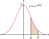
Numerical integration is the process of approximating a definite integral using well-chosen sums of function values. It is needed when we cannot find an antiderivative explicitly, as in the case of the Gaussian function \(f(x) = e^{-x^2/2}\) (Figure 7.23).
To approximate the definite integral \({\int_a^b\,f(x)\, dx}\), we fix a whole number \(N\) and divide \([a,b]\) into \(N\) subintervals of length \(\Delta x=({b-a})/{N}\). The endpoints of the subintervals (Figure 7.24) are \[\boxed{\bbox[#FAF8ED,5pt]{ x_0=a,\qquad x_1 = a+\Delta x,\qquad x_2 = a+2\Delta x,\qquad\dots, \qquad x_N = b }}\]
We shall denote the values of \(f(x)\) at these endpoints by \(y_j\): \[ \boxed{\bbox[#FAF8ED,5pt]{y_j = f(x_j)=f(a+j\Delta x)%\quad (j = 0, 1, 2, \dots , N) }}\]
In particular, \(y_0=f(a)\) and \(y_N=f(b)\).
The Trapezoidal Rule \(T_N\) approximates \({\int_a^b f(x)\,dx}\) by the area of the trapezoids obtained by joining the points \((x_0,y_0)\), \((x_1, y_1), \dots, (x_N,y_N)\) with line segments as in Figure 7.24. The area of the \(j\)th trapezoid is \(\frac12\Delta x(y_{j-1}+y_j)\), and therefore, \[ \begin{align*} T_N &= \frac12\Delta x(y_{0}+y_1)+\frac12\Delta x(y_1+y_2)+\cdots + \frac12\Delta x(y_{N-1}+y_N)\\ &= \frac12\Delta x\Big((y_{0}+y_1)+ (y_1+y_2)+\cdots + (y_{N-1}+y_N)\Big) \end{align*} \]
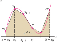
Note that each value \(y_j\) occurs twice except for \(y_0\) and \(y_N\), so we obtain \[ T_N = \frac12\Delta x\Big(y_{0}+2y_1 + 2y_2 +\cdots + 2y_{N-1}+y_N\Big) \]
Trapezoidal Rule
The \(N\)th trapezoidal approximation to \(\displaystyle\int_a^b f(x)\, dx\) is \[ \boxed{\bbox[#FAF8ED,5pt]{ T_N = \frac{1}{2}\,\Delta x \bigl(y_0 + 2y_1 + \cdots + 2y_{N-1} + y_N \bigr) }} \]
where \(\Delta x = \dfrac{b-a}{N}\) and \(y_j = f(a+j\,\Delta x)\).
CONCEPTUAL INSIGHT
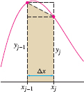
We see in Figure 7.25 that the area of the \(j\)th trapezoid is equal to the average of the areas of the endpoint rectangles with heights \(y_{j-1}\) and \(y_j\). It follows that \(T_N\) is equal to the average of the right- and left-endpoint approximations \(R_N\) and \(L_N\) introduced in Section 5.1: \[ T_N=\frac12(R_N+L_N) \]
In general, this average is a better approximation than either \(R_N\) alone or \(L_N\) alone.
455
EXAMPLE 1
![]() Calculate \(T_8\) for the integral \({ \int_1^{3} \sin(x^2)\, dx}\). Then use a computer algebra system to
calculate \(T_N\) for \(N = 50, 100, 500, 1000\), and \(10{,}000\).
Calculate \(T_8\) for the integral \({ \int_1^{3} \sin(x^2)\, dx}\). Then use a computer algebra system to
calculate \(T_N\) for \(N = 50, 100, 500, 1000\), and \(10{,}000\).
Solution Divide \([1,3]\) into \(N=8\) subintervals of length \(\Delta x = \frac{3-1}{8} = \frac{1}{4}\). Then sum the function values at the endpoints (Figure 7.26) with the appropriate coefficients: \[ \begin{eqnarray*} T_{8}&=& \frac12\left(\frac14\right)\big[\sin(1^2) + 2\sin(1.25^2) + 2\sin(1.5^2) + 2\sin(1.75^2)\\ &&\quad{}+ 2\sin(2^2) + 2\sin(2.25^2) + 2\sin(2.5^2) + 2\sin(2.75^2) + \sin(3^2)\big]\\ &\approx& 0.4281 \end{eqnarray*} \]
In general, \(\Delta x = (3-1)/N = 2/N\) and \(x_j = 1+ 2j/N\). In summation notation, \[ T_N = \frac12\left(\frac2N\right)\Biggl[\sin(1^2)+2 \underbrace{\sum_{j=1}^{N-1}\sin\left(\left(1+\frac{2j}N\, \right)^2\right)}_{\textrm{Sum of terms with coefficient \(2\)}}+\sin(3^2) \Biggr] \]
We evaluate the inner sum on a CAS, using a command such as
\(\mathtt{Sum[Sin[(1+2j/N)}\textrm{^}\)\(\mathtt{2], \{j, 1,N-1\}]}\)
| \(N\) | \(T_N\) |
| 50 | 0.4624205 |
| 100 | 0.4630759 |
| 500 | 0.4632855 |
| 1000 | 0.4632920 |
| 10,000 | 0.4632942 |
The results in Table 7.1 suggest that \({\int_1^3 \sin (x^2)\,dx}\) is approximately 0.4633.
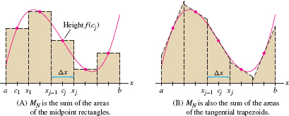
The midpoint approximation \(M_N\), introduced in Section 5.1, is the sum of the areas of the rectangles of height \(f(c_j)\) and base \(\Delta x\), where \(c_j\) is the midpoint of the interval \([x_{j-1},x_j]\) [Figure 7.28].
Midpoint Rule
The \(N\)th midpoint approximation to \(\displaystyle\int_a^b f(x)\, dx\) is \[ \boxed{\bbox[#FAF8ED,5pt]{ M_N = \Delta x \bigl( f(c_1) + f(c_2) +\cdots + f(c_N) \bigr)}} \]
where \(\Delta x = \dfrac{b-a}{N}\) and \(c_j = a + \big(j-\frac12\big)\,\Delta x\) is the midpoint of \([x_{j-1},x_j]\).
GRAPHICAL INSIGHT
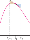
\(M_N\) has a second interpretation as the sum of the areas of tangential trapezoids—that is, trapezoids whose top edges are tangent to the graph of \(f(x)\) at the midpoints \(c_j\) [Figure 7.28]. The trapezoids have the same area as the rectangles because the top edge of the trapezoid passes through the midpoint of the top edge of the rectangle, as shown in Figure 7.27.
456
Error Bounds
In applications, it is important to know the accuracy of a numerical approximation. We define the error in \(T_N\) and \(M_N\) by \[ \text{Error}(T_N) = \left| \int_a^b f(x)\, dx - T_N\right|,\qquad \text{Error}(M_N) = \left| \int_a^b f(x)\, dx - M_N\right| \]
According to the next theorem, the magnitudes of these errors are related to the size of the second derivative \(f''(x)\). A proof of Theorem 1 is provided in a supplement on the text's Companion Web Site.
In the error bound, you can let \(K_2\) be the maximum of \(|f''(x)|\) on \([a,b]\), but if it is inconvenient to find this maximum exactly, take \(K_2\) to be any number that is definitely larger than the maximum.
THEOREM 1 Error Bound for \(T_N\) and \(M_N\)
Assume \(f''(x)\) exists and is continuous. Let \(K_2\) be a number such that \(|f''(x)| \le K_2\) for all \(x\in[a,b]\). Then \[ \boxed{\bbox[#FAF8ED,5pt]{\text{Error}(T_N) \le \frac{K_2(b- a)^3}{12N^2},\qquad \text{Error}(M_N) \le \frac{K_2(b- a)^3}{24N^2}}} \]
GRAPHICAL INSIGHT
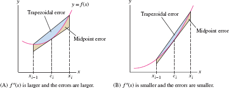
Note that the error bound for \(M_N\) is one-half of the error bound for \(T_N\), suggesting that \(M_N\) is generally more accurate than \(T_N\). Why do both error bounds depend on \(f''(x)\)? The second derivative measures concavity, so if \(|f''(x)|\) is large, then the graph of \(f\) bends a lot and trapezoids do a poor job of approximating the region under the graph. Thus the errors in both \(T_N\) and \(M_N\) (which uses tangential trapezoids) are likely to be large (Figure 7.29).
EXAMPLE 2 Checking the Error Bound
Calculate \(T_6\) and \(M_6\) for \(\displaystyle\int_1^4 \sqrt{x}\, dx\).
- Calculate the error bounds.
- Calculate the integral exactly and verify that the error bounds are satisfied.
Solution Divide \([1,4]\) into six subintervals of width \(\Delta x =\frac{4-1}{6} = \frac12\). Using the endpoints and midpoints shown in Figure 7.30, we obtain \[ \begin{align*} T_6&= \frac12\left(\frac12\right)\Big(\sqrt{1} + 2\sqrt{1.5} + 2\sqrt{2} + 2\sqrt{2.5} + 2\sqrt{3} + 2\sqrt{3.5} + \sqrt{4} \Big)\approx 4.661488 \\ M_6&= \frac12 \Big(\sqrt{1.25} + \sqrt{1.75} + \sqrt{2.25} + \sqrt{2.75} + \sqrt{3.25} + \sqrt{3.75}\Big) \approx 4.669245 \end{align*} \]
457
- Let \(f(x) = \sqrt x\). We must find a
number \(K_2\) such that \(|f''(x)|\le K_2\) for \(1\le x \le 4\). We
have \(f''(x)=-\frac14x^{-3/2}\). The absolute value \(|f''(x)|=\frac14x^{-3/2}\) is
decreasing on \([1,4]\), so its maximum occurs at
\(x=1\) (Figure 7.31). Thus, we may take \(K_2=|f''(1)|=\frac14\).
By Theorem 1,
\[
\begin{align*}
\text{Error}(T_6) &\le \frac{K_2(b- a)^3}{12N^2} =
\frac{\frac14(4-1)^3}{12(6)^2} =\frac1{64}\approx
0.0156
\\
\text{Error}(M_6) &\le \frac{K_2(b- a)^3}{24N^2} =
\frac{\frac14(4 - 1)^3}{24(6)^2} = \frac1{128} \approx 0.0078
\end{align*}
\]
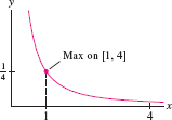 Figure 7.31: Graph of \(y=|f''(x)|=\frac14x^{-3/2}\) for \(f(x)=\sqrt x\).
In Example 2, the error in \(T_6\) is approximately twice as large as the error in \(M_6\). In practice, this is often the case.
- The exact value is \({\int_1^4 \sqrt{x}\, dx= \frac23 x^{3/2}\big|_1^4 = \frac{14}{3}}\), so the actual errors are
\[
\begin{alignat*}{3}
\text{Error}(T_6) & \approx&\: \left\vert \frac{14}3 - 4.661488 \right\vert&\approx 0.00518&\quad\textrm{(less than error bound \(0.0156\))}\\
\text{Error}(M_6) & \approx&\: \left\vert \frac{14}3 - 4.669245\right\vert&\approx 0.00258&\quad\textrm{(less than error bound \(0.0078\))}
\end{alignat*}
\]
The actual errors are less than the error bound, so Theorem 1 is verified.
The error bound can be used to determine values of \(N\) that provide a given accuracy.
EXAMPLE 3 Obtaining the Desired Accuracy
Find \(N\) such that \(T_N\) approximates \(\int_0^3 e^{-x^2}\, dx\) with an error of at most \(10^{-4}\).
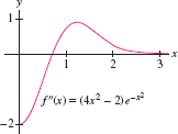
Solution Let \(f(x)=e^{-x^2}\). To apply the error bound, we must find a number \(K_2\) such that \(|f''(x)|\le K_2\) for all \(x\in [0,3]\). We have \(f'(x)=-2xe^{-x^2}\) and \[ f''(x) = (4x^2-2)e^{-x^2} \]
A quick way to find a value for \(K_2\) is to plot \(f''(x)\) using a graphing utility and find a bound for \(|f''(x)|\) visually, as we do in Example 3.
Let's use a graphing utility to plot \(f''(x)\) (Figure 7.32). The graph shows that the maximum value of \(|f''(x)|\) on \([0,3]\) is \(|f''(0)|=|-2|=2\), so we take \(K_2=2\) in the error bound: \[ \text{Error}(T_N) \le \frac{K_2(b-a)^3}{12N^2} = \frac{2(3-0)^3}{12 N^2} = \frac{9}{2N^2} \]
The error is at most \(10^{-4}\) if \[ \frac{9}{2N^2} \le 10^{-4}\quad\Rightarrow\quad N^2\ge \frac{9\times 10^4}{2}\quad\Rightarrow\quad N\ge \frac{300}{\sqrt{2}}\approx 212.1 \]
We conclude that \(T_{213}\) has error at most \(10^{-4}\). We can confirm this using a computer algebra system. A CAS shows that \(T_{213} \approx 0.886207\), whereas the value of the integral to nine places is \(0.886207348\). Thus the error is less than \(10^{-6}\).
Can we improve on the Trapezoidal and Midpoint Rules? One clue is that the exact value of the integral lies between \(T_N\) and \(M_N\) if \(f(x)\) is concave up or down. In fact, we see geometrically (Figure 7.33) that
- \(f(x)\) is concave down\(\quad\)\(\Rightarrow\)\(\quad\) \(\phantom{M_N}\llap{T_N}\le \displaystyle\int_a^b f(x)\,dx \le M_N\).
- \(f(x)\) is concave up\(\quad\) \(\Rightarrow\)\(\quad\) \(\displaystyle M_N\le \int_a^b f(x)\,dx\le T_N\).
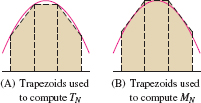
This suggests that the errors in \(T_N\) and \(M_N\) may cancel partially if we take their average.
458
Simpson's Rule exploits this idea, but it takes into account that \(M_N\) is roughly twice as accurate as \(T_N\). To minimize the error, Simpson's Rule \(S_N\) is defined as a weighted average that uses twice as much \(M_N\) as \(T_N\). For \(N\) even, let \[ S_N = \frac13\,T_{N/2} + \frac23\,M_{N/2}\tag{1} \]
To derive a formula for \(S_N\), we divide \([a,b]\) into \(N\) subintervals as usual. Observe that the even-numbered endpoints divide \([a,b]\) into \(N/2\) subintervals of length \(2\Delta x\) (keep in mind that \(N\) is even): \[ \label{8.numint.intervals} [x_0,x_2],\,\,\, [x_2,x_4],\,\,\, \dots,\,\,\, [x_{N-2},x_N]\tag{2} \]
The endpoints of these intervals are \(x_0, x_2, \ldots, x_N\). They are used to compute \(T_{N/2}\). The midpoints \(x_1, x_3, \ldots, x_{N-1}\) are used to compute \(M_{N/2}\) (see Figure 7.34 for the case \(N = 8\)). \[ \begin{align*} T_{N/2} &= \frac12(2\Delta x) \big(y_0+2y_2+2y_4+\cdots + 2y_{N-2}+y_{N} \big)\\ M_{N/2} &= 2\Delta x\big(y_1+y_3 + y_5 + \cdots +y_{N-1} \big) = \Delta x\big(2y_1+2y_3 + 2y_5 + \cdots +2y_{N-1} \big) \end{align*} \]

Thus, \[ \begin{eqnarray*} S_N = \frac13 T_{N/2}+\frac23 M_{N/2} &=& \frac13\Delta x \big(y_0+2y_2+2y_4+\cdots + 2y_{N-2}+y_{N} \big)\\ &&{} + \frac13\Delta x\big(4y_1+4y_3 + 4y_5 + \cdots +4y_{N-1} \big) \end{eqnarray*} \]
Pattern of coefficients in \(S_N\): \[ 1, 4, 2, 4, 2, 4, \ldots, 4, 2, 4, 1 \]
The intermediate coefficients alternate \(4, 2, 4, 2,\dots , 2, 4\) (beginning and ending with \(4\)).
Simpson's Rule
For \(N\) even, the \(N\)th approximation to \(\displaystyle\int_a^b f(x)\, dx\) by Simpson's Rule is \[ S_N = \frac13\Delta x \bigl[y_0 + 4y_1 + 2y_2 + \cdots + 4y_{N-3} + 2y_{N-2} + 4y_{N-1} + y_N \bigr]\tag{3} \]
where \(\Delta x = \dfrac{b-a}{N}\) and \(y_j=f(a+j\,\Delta x)\).
CONCEPTUAL INSIGHT
Both \(T_N\) and \(M_N\) give the exact value of the integral for all \(N\) when \(f(x)\) is a linear function (Exercise 59). However, of all combinations of \(T_{N/2}\) and \(M_{N/2}\), only the particular combination \(S_N = \frac13T_{N/2}+\frac23M_{N/2}\) gives the exact value for all quadratic polynomials (Exercises 60 and 61). In fact, \(S_N\) is also exact for all cubic polynomials (Exercise 62).
EXAMPLE 4
Use Simpson's Rule with \(N = 8\) to approximate \(\displaystyle\int_2^4 \sqrt{1+x^3} \, dx\).
Solution We have \(\Delta x = \tfrac{4-2}8=\tfrac14\). Figure 7.35 shows the endpoints and coefficients needed to compute \(S_8\) using Eq. (3): \[ \begin{align*} \frac13\left(\frac14\right)& \bigl[\sqrt{1+2^3} + 4\sqrt{1+2.25^3} + 2\sqrt{1+2.5^3} + 4\sqrt{1+2.75^3} + 2\sqrt{1+3^3} \\ &+ 4\sqrt{1+3.25^3} + 2\sqrt{1+3.5^3} + 4\sqrt{1+3.75^3} +\sqrt{1+4^3} \bigr] \\ \approx \frac1{12} &\bigl[3 + 4(3.52003) + 2(4.07738) + 4( 4.66871) + 2(5.2915) \\ &+ 4(5.94375)+ 2(6.62382) + 4(7.33037) + 8.06226\bigr] \approx 10.74159 \end{align*} \]
The accuracy of Simpson's Rule is impressive. Using a computer algebra system, we find that the approximation in Example 4 has an error of less than \(3\times 10^{-6}\).
459
EXAMPLE 5 Estimating Integrals from Numerical Data
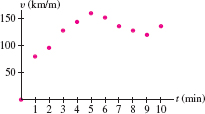
The velocity (in km/h) of a Piper Cub aircraft traveling due west is recorded every minute during the first 10 minutes after takeoff. Use Simpson's Rule to estimate the distance traveled.
| \(t\) (min) | 0 | 1 | 2 | 3 | 4 | 5 | 6 | 7 | 8 | 9 | 10 |
| \(v(t)~\text{(km/h)}\) | 0 | 80 | 100 | 128 | 144 | 160 | 152 | 136 | 128 | 120 | 136 |
Solution The distance traveled is the integral of velocity. We convert from minutes to hours because velocity is given in km/h, and thus we apply Simpson's Rule, where the number of intervals is \(N=10\) and each interval has length \(\Delta t = \frac{1}{60}\) hours: \[ \begin{eqnarray*} S_{10} &=& \left(\frac13\right)\left(\frac{1}{60}\right)\big(0\begin{array}[t]{@{}l@{}} {}+4(80)+2(100)+4(128)+2(144)+4(160)\\ {}+2(152)+4(136)+2(128)+4(120)+136\big)\approx 21.2\,\,\textrm{km}\end{array} \end{eqnarray*} \]
The distance traveled is approximately 21.2 km (Figure 7.36).
We now state (without proof) the error bound for Simpson's Rule. Set \[ \textrm{Error}(S_N) = \left\vert \int_a^b f(x) - S_N(f)\, dx \right\vert \]
The error involves the fourth derivative, which we assume exists and is continuous.
THEOREM 2 Error Bound for \(S_N\)
Let \(K_4\) be a number such that \(|f^{(4)}(x)| \le K_4\) for all \(x\in[a,b]\). Then \[ \boxed{\bbox[#FAF8ED,5pt]{\textrm{Error}(S_N) \le \frac{K_4(b- a)^5}{180 N^4}}} \]
Although Simpson's Rule provides good approximations, more sophisticated techniques are implemented in computer algebra systems. These techniques are studied in the area of mathematics called numerical analysis.
EXAMPLE 6
Calculate \(S_8\) for \(\displaystyle\int_1^{3}\dfrac{1}{x}\, dx\). Then:
- Find a bound for the error in \(S_8\).
- Find \(N\) such that \(S_N\) has an error of at most \(10^{-6}\).
Solution The width is \(\Delta x = \tfrac{3-1}{8}=\tfrac14\) and the endpoints in the partition of \([1,3]\) are \(1, 1.25, 1.5, \ldots , 2.75, 3\). Using Eq. (3) with \(f(x)=x^{-1}\), we obtain \[ \begin{eqnarray*} S_8 &=& \frac13\left(\frac14\right)\left[ \dfrac{1}{1} + \dfrac{4}{1.25} + \dfrac{2}{1.5} + \dfrac{4}{1.75} + \dfrac{2}{2} + \dfrac{4}{2.25} + \dfrac{2}{2.5} + \dfrac{4}{2.75} + \dfrac{1}{3} \right]\\ &\approx& 1.09873 \end{eqnarray*} \]
- The fourth derivative \(f^{(4)}(x) = 24x^{-5}\) is decreasing, so the max
of \(|f^{(4)}(x)|\) on \([1,3]\) is \(|f^{(4)}(1)| = 24\). Therefore, we use the error bound with \(K_4=24\):
\[
\begin{align*}
\textrm{Error}(S_N) &\le \frac{K_4(b- a)^5}{180 N^4} =\frac{24(3-1)^5}{180N^4} =
\frac{64}{15N^4}\\
\textrm{Error}(S_8) &\le \frac{K_4(b- a)^5}{180 (8)^4} =
\frac{24(3-1)^5}{180(8^4)} \approx 0.001
\end{align*}
\]
460
- The error will be at most \(10^{-6}\) if \(N\) satisfies
\[
\mathrm{Error}(S_N) = \frac{64}{15N^4} \le 10^{-6}
\]
In other words, \[ N^4\ge 10^6\left(\dfrac{64}{15}\right)\qquad\hbox{or}\qquad N\ge \left(\dfrac{10^6\cdot 64}{15}\right)^{1/4} \approx 45.45 \]
Thus, we may take \(N = 46\) (see marginal comment).
Using a CAS, we find that \[ \begin{eqnarray*} S_{46}&\approx& 1.09861241\\ \int_1^{3}\dfrac{1}{x}\, dx= \ln 3 &\approx& 1.09861229 \end{eqnarray*} \]
The error is indeed less than \(10^{-6}\).
GRAPHICAL INSIGHT
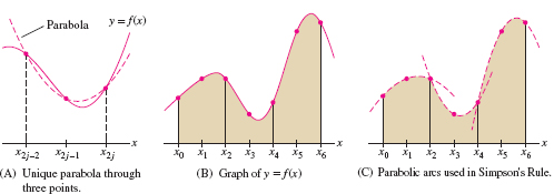
Simpson's Rule has an interpretation in terms of parabolas (Figure 7.37). There is a unique parabola passing through the graph of \(f(x)\) at the three points \(x_{2j-2}, x_{2j-1}, x_{2j}\) [Figure 7.37]. On the interval \([x_{2j-2}, x_{2j}]\), the area under the parabola approximates the area under the graph. Simpson's Rule \(S_N\) is equal to the sum of these parabolic approximations (see Exercises 60–61).
7.8.1 Summary
- We consider three numerical approximations to \(\int_a^b f(x) dx\): the Trapezoidal Rule \(T_N\), the Midpoint
Rule \(M_N\), and Simpson's Rule \(S_N\) (for \(N\) even).
\[
\begin{align*}
T_N &= \frac12\,\Delta x \big(y_0+2y_1+2y_2+\cdots +
2y_{N-1}+y_N\big)\\
M_N &= \Delta x \big( f(c_1) + f(c_2) +\cdots
+ f(c_N) \big)\qquad \left(c_j=a+\left(j-\frac12\right)\Delta x\right)
\\
S_N& = \frac13\Delta x \bigl[y_0 + 4y_1 +
2y_2 + \cdots + 4y_{N-3} + 2y_{N-2} + 4y_{N-1} +
y_N \bigr]
\end{align*}
\]
where \(\Delta x = ({b - a})/{N}\) and \(y_j = f(a + j\,\Delta x)\).
- \(T_N\) is equal to the sum of the areas of the trapezoids obtained by connecting the points \((x_0,y_0)\), \((x_1, y_1), \dots, (x_N,y_N)\) with line segments.
- \(M_N\) has two geometric interpretations; it may be interpreted either as the sum of the areas of the midpoint rectangles or as the sum of the areas of the tangential trapezoids.
- \(S_N\) is equal to \(\frac13 T_{N/2} + \frac23 M_{N/2}\).
- Error bounds: \[ \text{Error}(T_N) \le \frac{K_2(b- a)^3}{12N^2},\qquad\!\!\! \text{Error}(M_N) \le \frac{K_2(b- a)^3}{24N^2},\qquad\!\!\! \text{Error}(S_N) \le \frac{K_4(b- a)^5}{180N^4} \] where \(K_2\) is any number such that \(|f''(x)| \le K_2\) for all \(x\in[a,b]\) and \(K_4\) is any number such that \(|f^{(4)}(x)|\le K_4\) for all \(x\in [a,b]\).
461