8.4 Linear Approximation and Taylor Polynomials
The material in this section sets the stage for our next big topic in Chapter 10: Infinite series and Taylor series. We start with the linear approximation (or first-order approximation) to a function \(y=f(x)\) centered at a point \(x=a\) and then extend this to Taylor Polynomials of degree \(n\) which are approximations to order \(n\).
8.4.1 Linear Approximation
In some situations we are interested in determining the “effect of a small change.” For example:
- How does a small change in angle affect the distance of a basketball shot?
- How are revenues at the box office affected by a small change in ticket prices?
- The cube root of 27 is 3. How much larger is the cube root of 27.2?
In each case, we have a function \(f(x)\) and we’re interested in the change
\[ \boxed{\Delta f = f(a+\Delta x) - f(a)} \]
where \(\Delta x\) is small. The Linear Approximation uses the derivative to estimate \(\Delta f\) without computing it exactly. By definition, the derivative is the limit
\[ f'(a) = \lim\limits_{\Delta x\rightarrow 0}\frac{f(a+\Delta x) - f(a)}{\Delta x} = \lim\limits_{\Delta x\rightarrow 0}\frac{\Delta f}{\Delta x} \]
So when \(\Delta x\) is small, we have \(\frac{\Delta f}{\Delta x} \approx f'(a)\), and thus,
\[ \Delta f \approx f'(a)\Delta x \]
![]() REMINDER The notation \(\approx\) means “approximately equal to.” The accuracy of the Linear Approximation is discussed at the end of this section.
REMINDER The notation \(\approx\) means “approximately equal to.” The accuracy of the Linear Approximation is discussed at the end of this section.
Linear Approximation of Δf
If \(f\) is differentiable at \(x = a\) and \(\Delta x\) is small, then
\[ \boxed{\Delta f \approx f'(a)\Delta x}\tag{1} \]
where \(\Delta f = f(a + \Delta x) - f(a)\).
Keep in mind the different roles played by \(\Delta f\) and \(f'(a)\Delta x\). The quantity of interest is the actual change \(\Delta f\). We estimate it by \(f'(a) \Delta x\). The Linear Approximation tells us that up to a small error, \(\Delta f\) is directly proportional to \(\Delta x\) when \(\Delta x\) is small.
208
GRAPHICAL INSIGHT
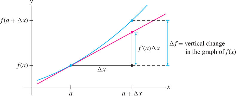
The Linear Approximation is sometimes called the tangent line approximation. Why? Observe in Figure 8.33 that \(\Delta f\) is the vertical change in the graph from \(x = a\) to \(x = a + \Delta x\). For a straight line, the vertical change is equal to the slope times the horizontal change \(\Delta x\), and since the tangent line has slope \(f'(a)\), its vertical change is \(f'(a)\Delta x\). So the Linear Approximation approximates \(\Delta f\) by the vertical change in the tangent line. When \(\Delta x\) is small, the two quantities are nearly equal.
EXAMPLE 1
Linear Approximation:
\[ \Delta f \approx f'(a)\Delta x \]
where\( \Delta f = f(a + \Delta x) - f(a)\)
Use the Linear Approximation to estimate \(\frac{1}{10.2} - \frac{1}{10}\). How accurate is your estimate?
Solution We apply the Linear Approximation to \(f(x)=\frac{1}{x}\) with \(a = 10\) and \(\Delta x = 0.2\):
\[ \Delta f = f(10.2) - f(10) = \frac{1}{10.2} - \frac{1}{10} \]
We have \(f'(x) = -x^{-2}\)and\( f'(10) = -0.01\), so \(\Delta f\) is approximated by
\[ f'(10)\Delta x = (-0.01)(0.2) = -0.002 \]
In other words,
\[ \frac{1}{10.2} - \frac{1}{10} \approx -0.002 \]
The error in the Linear Approximation is the quantity
\[ \text{Error} = |\Delta f - f'(a)\Delta x| \]
A calculator gives the value \(\frac{1}{10.2} - \frac{1}{10} \approx -0.00196\) and thus our error is less than \(10^{-4}\):
\[ \text{Error} \approx |-0.00196 -(-0.002)| = 0.00004 < 10^{-4} \]
Question 8.3 Linear Approximation Progress Check Question 1
Use the linear approximation to estimate \( \sin(.03)-\sin(0)= \sin(.03)-0= \sin(.03)\)
Differential Notation
The Linear Approximation to \(y = f(x)\) is often written using the “differentials” \(dx\) and \(dy\). In this notation, \(dx\) is used instead of \(\Delta x\) to represent the change in \(x\), and \(dy\) is the corresponding vertical change in the tangent line:
\[ \boxed{dy = f'(a)dx}\tag{2} \]
Let \(\Delta y = f(a + dx) - f(a)\). Then the Linear Approximation says
\[\boxed{\Delta y\approx dy}\tag{3}\]
This is simply another way of writing \(\Delta f \approx f'(a)\Delta x\).
EXAMPLE 2 Differential Notation
Approximately how much larger is \(\sqrt[3]{8.1}\) than \(\sqrt[3]{8} = 2\)?
Solution We are interested in \(\sqrt[3]{8.1} - \sqrt[3]{8}\), so we apply the Linear Approximation to \(f(x) = x^{\frac{1}{3}}\) with \(a = 8\) and change \(\Delta x = dx = 0.1\).
209
Step 1. Write out \(\Delta y\).
\[ \Delta y = f(a+dx) - f(a) =\sqrt[3]{8+0.1} - \sqrt[3]{8} = \sqrt[3]{8.1} - 2 \]
Step 2. Compute \(dy\).
\[ f'(x) = \frac{1}{3}x^{-\frac{2}{3}}\text{ and }f'(8)=\left(\frac{1}{3}\right)8^{-\frac{2}{3}} = \left(\frac{1}{3}\right)\left(\frac{1}{4}\right)=\frac{1}{12} \]
Therefore, \(dy = f'(8)dx =\frac{1}{12}(0.1)\approx 0.0083\).
Step 3. Use the Linear Approximation.
\[ \Delta y\approx dy\implies \sqrt[3]{8.1} - 2 \approx 0.0083 \]
Thus \(\sqrt[3]{8.1}\) is larger than \(\sqrt[3]{8}\) by approximately 0.0083, and \(\sqrt[3]{8.1}\approx2.0083\).
When engineers need to monitor the change in position of an object with great accuracy, they may use a cable position transducer (Figure 8.34). This device detects and records the movement of a metal cable attached to the object. Its accuracy is affected by changes in temperature because heat causes the cable to stretch. The Linear Approximation can be used to estimate these effects.

EXAMPLE 3 Thermal Expansion
A thin metal cable has length \(L = 12\text{ cm}\) when the temperature is \(T = 21^\circ\text{C}\). Estimate the change in length when \(T\) rises to 24°C, assuming that
\[ \frac{dL}{dT} = kL\tag{4} \]
where \(k = 1.7 \times10^{-5}(^\circ\text{C})^{-1}\) (\(k\) is called the coefficient of thermal expansion).
Solution How does the Linear Approximation apply here? We will use the differential \(dL\) to estimate the actual change in length \(\Delta L\) when \(T\) increases from 21° to 24°—that is, when \(dT = 3^\circ\). By Eq. (2), the differential \(dL\) is
\[ dL = \left(\frac{dL}{dT}\right)dT \]
By Eq. (4), since \(L = 12\),
\[ \left.\frac{dL}{dT}\right|_{L=12} = k L = (1.7 \times10^{-5})(12) \approx 2\times 10^{-4}\text{ cm/\(^\circ\)C} \]
The Linear Approximation \(\Delta L \approx dL\) tells us that the change in length is approximately
\[ \Delta L \approx\underbrace{\left(\frac{dL}{dT}\right)dT}_{dL}\approx(2\times 10^{-4})(3) = 6\times 10^{-4}\text{ cm} \]
Suppose that we measure the diameter D of a circle and use this result to compute the area of the circle. If our measurement of D is inexact, the area computation will also be inexact. What is the effect of the measurement error on the resulting area computation? This can be estimated using the Linear Approximation, as in the next example.
EXAMPLE 4 Effect of an Inexact Measurement
The Bonzo Pizza Company claims that its pizzas are circular with diameter 50 cm (Figure 8.35).

(a) What is the area of the pizza?
(b) Estimate the quantity of pizza lost or gained if the diameter is off by at most 1.2 cm.
210
Solution First, we need a formula for the area \(A\) of a circle in terms of its diameter \(D\). Since the radius is \(r = \frac{D}{2}\), the area is
\[ A(D) = \pi r^2 = \pi\left(\frac{D}{2}\right)^2 = \frac{\pi}{4}D^2 \]
(a) If \(D = 50\text{ cm}\), then the pizza has area \(A(50) = \left(\frac{\pi}{4}\right)(50)^2\approx1963.5\text{ cm}^2\).
In this example, we interpret \(\Delta A\) as the possible error in the computation of \(A(D)\). This should not be confused with the error in the Linear Approximation. This latter error refers to the accuracy in using \(A'(D) \Delta D\) to approximate \(\Delta A\).
(b) If the actual diameter is equal to \(50 + \Delta D\), then the loss or gain in pizza area is \(\Delta A = A(50 + \Delta D) - A(50)\). Observe that \(A'(D) = \frac{\pi}{2}D\) and \(A'(50) = 25\pi \approx 78.5\text{ cm}\), so the Linear Approximation yields
\[ \Delta A = A(50 + \Delta D) - A(50) \approx A'(D)\Delta D \approx (78.5) \Delta D \]
Because \(\Delta D\) is at most \(\pm 1.2 \text{ cm}\), the loss or gain in pizza is no more than around
\[ \Delta A \approx \pm (78.5)(1.2) \approx \pm 94.2\text{ cm}^{2} \]
This is a loss or gain of approximately \(4.8\%\).
To approximate the function \(f(x)\) itself rather than the change \(\Delta f\), we use the linearization \(L(x)\) “centered at \(x = a\),” defined by
\[ L(x) = f'(a)(x - a) + f(a) \]
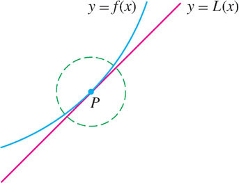
Notice that \(y = L(x)\) is the equation of the tangent line at \(x = a\) (Figure 8.36). If \(f(x)\) is differentiable at \(x=a\), then for values of \(x\) close to \(a\), \(L(x)\) provides a good approximation to \(f(x)\).
Approximating f(x) by Its Linearization
If \(f\) is differentiable at \(x = a\) and \(x\) is close to \(a\), then
\[ \boxed{f(x)\approx L(x) = f'(a)(x - a) + f(a)} \]
CONCEPTUAL INSIGHT
Keep in mind that the linearization and the Linear Approximation are two ways of saying the same thing. Indeed, when we apply the linearization with \(x = a + \Delta x\) and re-arrange, we obtain the Linear Approximation:
\begin{align*} f(x)&\approx f(a) + f'(a)(x-a)\\ f(a + \Delta x) &\approx f(a) + f'(a)\Delta x\quad(\text{since }\Delta x = x-a)\\ f(a + \Delta x) - f(a)&\approx f'(a)\Delta x \end{align*}
EXAMPLE 5
Compute the linearization of \(f(x) = \sqrt{x}e^{x-1}\) centered at \(a = 1\).
Solution By the Product Rule:
\begin{gather*} f'(x) = x^{\frac{1}{2}}e^{x-1} + \frac{1}{2}x^{-\frac{1}{2}}e^{x-1} = \left(x^{\frac{1}{2}} + \frac{1}{2}x^{-\frac{1}{2}}\right)e^{x-1}\\ f(1) = \sqrt1e^0=1\quad f'(1)=\left(1+\frac{1}{2}\right)e^0 = \frac{3}{2} \end{gather*}
Therefore, the linearization at \(a = 1\) is
\[ L(x) = f(1) + f'(1)(x-1) = 1 + \frac{3}{2}(x-1)=\frac{3}{2}x - \frac{1}{2} \]
Question 8.4 Linear Approximation Progress Check 2
Find the linearization \(L(x)\) of \(f(x) = 2x \cos x+1\) at \(x=0\). Give your answer in the form L=mx+b, NO SPACES.
211
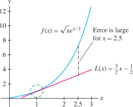
The linearization can be used to approximate function values. The following table compares values of the linearization to values obtained from a calculator for the function \(f(x) = \sqrt{x}e^{x-1}\) in the previous example. Note that the error is large for \(x = 2.5\), as expected, because 2.5 is not close to the center \(a = 1\) (Figure 8.37).
| \(x\) | \(\sqrt{x}e^{x-1}\) | Linearization at \(a = 1\): \(L(x) = \frac{3}{2}x - \frac{1}{2}\) | Calculator | Error |
|---|---|---|---|---|
| \(1.1\) | \(\sqrt{1.1}e^{0.1}\) | \(L(1.1) = \frac{3}{2}(1.1) - \frac{1}{2} = 1.15\) | \(1.15911\) | \(10^{-2}\) |
| \(0.999\) | \(\sqrt{0.999}e^{-0.001}\) | \(L(0.999) = \frac{3}{2}(0.999) - \frac{1}{2} = 0.9985\) | \(0.998501\) | \(10^{-6}\) |
| \(2.5\) | \(\sqrt{2.5}e^{1.5}\) | \(L(2.5) = \frac{3}{2}(2.5) - \frac{1}{2} = 3.75\) | \(7.086\) | \(3.84\) |
In the next example, we compute the percentage error, which is often more important than the error itself. By definition,
\[ \boxed{\text{Percentage error}=\left|\dfrac{\text{error}}{\text{actual value}}\right|\times100\%} \]
EXAMPLE 6
Estimate \(\tan(\frac{\pi}{4}+0.02)\) and compute the percentage error.
Solution We find the linearization of \(f(x)=\tan x\) at \(a=\frac{\pi}{4}\):
\begin{gather*} f\left(\frac{\pi}{4}\right) = \tan\left(\frac{\pi}{4}\right) = 1\quad f'\left(\frac{\pi}{4}\right)=\sec^2\left(\frac{\pi}{4}\right) = (\sqrt{2})^2=2\\ L(x) = f\left(\frac{\pi}{4}\right) + f'\left(\frac{\pi}{4}\right)\left(x-\frac{\pi}{4}\right) = 1 + 2\left(x-\frac{\pi}{4}\right) \end{gather*}
At \(x=\frac{\pi}{4}+0.02\), the linearization yields the estimate
\[ \tan\left(\frac{\pi}{4}+0.02\right)\approx L\left(\frac{\pi}{4}+0.02\right) = 1 + 2(0.02) = 1.04 \]
A calculator gives \(\tan\left(\frac{\pi}{4}+0.02\right)\approx1.0408\), so
\[ \text{Percentage error}\approx\left|\frac{1.0408 - 1.04}{1.0408}\times 100 \approx 0.08\%\right| \]
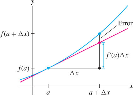
The examples in this section may have convinced you that the Linear Approximation yields a good approximation to \(\Delta f\) when \(\Delta x\) is small, but if we want to rely on the Linear Approximation, we need to know more about the size of the error:
\[ E = \text{Error} = |\Delta f - f'(a)\Delta x| \]
Remember that the error \(E\) is simply the vertical gap between the graph and the tangent line (Figure 8.38). In Section 10.7, we will prove the following Error Bound:
\[ \boxed{E\leq \dfrac{1}{2}K(\Delta x)^2}\tag{5} \]
where \(K\) is the maximum value of \(|f''(x)|\) on the interval from \(a\) to \(a + \Delta x\).
212
Error Bound:
\[ \boxed{E\leq \dfrac{1}{2}K(\Delta x)^2}\tag{5} \]
where \(K\) is the max of \(|f''|\) on the interval \([a, a + \Delta x]\).
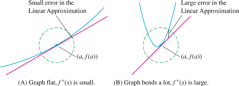
The Error Bound tells us two important things. First, it says that the error is small when the second derivative (and hence \(K\)) is small. This makes sense, because \(f''(x)\) measures how quickly the tangent lines change direction. When \(|f''(x)|\) is smaller, the graph is flatter and the Linear Approximation is more accurate over a larger interval around \(x = a\) (compare the graphs in Figure 8.39).
Second, the Error Bound tells us that the error is of order two
8.4.2 Taylor Polynomials
In Section 4.1, we used the linearization \(L(x)\) to approximate a function \(f(x)\) near a point \(x = a\): \[ L(x) = f(a) + f'(a)(x - a) \]

We refer to \(L(x)\) as a “first-order” approximation to \(f(x)\) at \(x=a\) because \(f(x)\) and \(L(x)\) have the same value and the same first derivative at \(x=a\) (Figure 8.40): \[ L(a) = f(a),\qquad L'(a) = f'(a) \]
A first-order approximation is useful only in a small interval around \(x = a\). In this section we learn how to achieve greater accuracy over larger intervals using the higher-order approximations (Figure 8.41).


In what follows, assume that \(f(x)\) is defined on an open interval \(I\) and that all higher derivatives \(f^{(k)}(x)\) exist on \(I\). Let \(a\in I\). We say that two functions \(f(x)\) and \(g(x)\) agree to order n at \(x=a\) if their derivatives up to order \(n\) at \(x=a\) are equal: \[ f(a)=g(a),\quad f^{\prime }(a)=g^{\prime }(a),\quad f^{\prime \prime }(a)=g^{\prime \prime }(a),\quad\ldots ,\quad f^{(n)}(a)=g^{(n)}(a) \]
We also say that \(g(x)\) “approximates \(f(x)\) to order \(n\)” at \(x=a\).
Define the \(n\)th Taylor polynomial centered at \(x=a\) as follows: \[ \boxed{\bbox[#FAF8ED,5pt]{ T_{n}(x)=f(a)+\frac{f^{\prime }(a)}{1!}(x-a) +\frac{f^{\prime \prime }(a)}{2!}(x-a)^{2}+\cdots +\frac{f^{(n)}(a)}{n!}(x-a)^{n} }} \]
The first few Taylor polynomials are \[ \begin {eqnarray} T_{0}(x) &=&f(a)\notag \\ T_{1}(x) &=&f(a)+f^{\prime }(a)(x-a)\notag \end {eqnarray}\]
489
\[ \begin {eqnarray} T_{2}(x) &=&f(a)+f^{\prime }(a)(x-a)+\frac{1}{2}f^{\prime \prime }(a)(x-a)^{2}\notag \\ T_{3}(x) &=&f(a)+f^{\prime }(a)(x-a)+\frac{1}{2}f^{\prime \prime }(a)(x-a)^2+\frac{1}{6}f^{\prime \prime \prime }(a)(x-a)^3 \notag\end {eqnarray}\]
Note that \(T_{1}(x)\) is the linearization of \(f(x)\) at \(a\). Note also that \(T_{n}(x)\) is obtained from \(T_{n-1}(x)\) by adding on a term of degree \(n\): \[\boxed{\bbox[#FAF8ED,5pt]{ T_n(x) = T_{n-1}(x) + \frac{f^{(n)}(a)}{n!}(x-a)^{n} }}\]
The next theorem justifies our definition of \(T_n(x)\).
Reminder
\(k\)-factorial is the number \(k! = k(k-1)(k-2)\cdots (2)(1)\). Thus, \[ \begin{align*} 1!=1,\quad 2!=(2)1 = 2\\ 3!=(3)(2)1 =6 \end{align*} \]
By convention, we define \(0! = 1\).
THEOREM 1
The polynomial \(T_n(x)\) centered at \(a\) agrees with \(f(x)\) to order \(n\) at \(x = a\), and it is the only polynomial of degree at most \(n\) with this property.
The verification of Theorem 1 is left to the exercises (Exercises 70-71), but we'll illustrate the idea by checking that \(T_2(x)\) agrees with \(f(x)\) to order \(n=2\). \[ \begin{eqnarray*} T_{2}(x)&=&f(a)+f^{\prime }(a)(x-a)+\frac{1}{2}f^{\prime \prime }(a)(x-a)^{2}, & T_{2}(a)&=&f(a) \\ T_{2}^{\prime }(x)&=&f^{\prime }(a)+f^{\prime \prime }(a)(x-a), & T_{2}^{\prime }(a)&=&f^{\prime }(a) \\ T_{2}^{\prime \prime }(x)&=&f^{\prime \prime }(a), & T_{2}^{\prime \prime}(a)&=&f^{\prime \prime }(a \end{eqnarray*} \]
This shows that the value and the derivatives of order up to \(n=2\) at \(x=a\) are equal. Before proceeding to the examples, we write \(T_n(x)\) in summation notation: \[\boxed{\bbox[#FAF8ED,5pt]{ T_{n}(x)=\sum \limits_{j=0}^{n} \frac{f^{(j)}(a)}{j!}\ (x-a)^{j} }}\]
By convention, we regard \(f(x)\) as the zeroeth derivative, and thus \(f^{(0)}(x)\) is \(f(x)\) itself. When \(a=0\), \(T_n(x)\) is also called the \(n\)th Maclaurin polynomial.
EXAMPLE 7 Maclaurin Polynomials for \(e^x\)
Plot the third and fourth Maclaurin polynomials for \(f(x)=e^x\). Compare with the linear approximation.
Solution All higher derivatives coincide with \(f(x)\) itself: \(f^{(k)}(x) = e^x\). Therefore, \[ f(0) = f'(0) = f''(0) = f'''(0) = f^{(4)}(0) = e^0 = 1 \]
The third Maclaurin polynomial (the case \(a = 0\)) is \[ T_3(x) = f(0) + f'(0)x + \frac12f''(0)x^2 + \frac1{3!}f'''(0)x^3 = 1 + x + \frac12x^2+\frac16x^3\\\]
We obtain \(T_4(x)\) by adding the term of degree 4 to \(T_3(x)\): \[ T_4(x) = T_3(x) + \frac1{4!}f^{(4)}(0)x^4 = 1 + x + \frac12x^2+\frac16x^3 + \frac1{24}x^4 \]
Figure 8.42 shows that \(T_3\) and \(T_4\) approximate \(f(x) = e^x\) much more closely than the linear approximation \(T_1(x)\) on an interval around \(a=0\). Higher-degree Taylor polynomials would provide even better approximations on larger intervals.

Question 8.5 Taylor Polynomials Progress Check Question 1
Compute the Taylor polynomial \(T_3(x)\) centered at \(a=0\) for \(f(x)=\tan{x}\).
| A. |
| B. |
| C. |
| D. |
| E. |
490
EXAMPLE 8 Computing Taylor Polynomials
Compute the Taylor polynomial \(T_4(x)\) centered at \(a=3\) for \(f(x)=\sqrt{x+1}\).
Solution First evaluate the derivatives up to degree 4 at \(a=3\): \[ \begin{eqnarray*} f(x) &=& (x+1)^{1/2}, \quad\quad\quad\quad& f(3)&=&2 \\[3pt] f^{\prime }(x) &=&\frac{1}{2}(x+1)^{-1/2}, & f^{\prime }(3)&=&\frac{1}{4} \\[3pt] f''(x) &=& -\frac{1}{4}(x+1)^{-3/2}, & f''(3)&=&-\frac{1}{32} \\[3pt] f'''(x) &=&\frac{3}{8}(x+1)^{-5/2}, & f'''(3)&=& \frac{3}{256} \\[3pt] f^{(4)}(x) &=& -\frac{15}{16}(x+1)^{-7/2}, & f^{(4)}(3)&=& -\frac{15}{2048} \end{eqnarray*} \]
Then compute the coefficients \(\frac{f^{(j)}(3)}{j!}\): \[ \begin{alignat*}{3} &\textrm{Constant term}&& = f(3) = 2 \\ &\textrm{Coefficient of $(x-3)$}&& = f'(3)=\frac14\\ &\textrm{Coefficient of $(x-3)^2$}&& = \frac{f''(3)}{2!} = -\frac{1}{32}\cdot\frac1{2!}=-\frac1{64}\\[3pt] &\textrm{Coefficient of $(x-3)^3$}&& = \frac{f'''(3)}{3!} = \frac{3}{256}\cdot\frac1{3!} = \frac1{512}\\[3pt] &\textrm{Coefficient of $(x-3)^4$}&& = \frac{f^{(4)}(3)}{4!} =- \frac{15}{2048}\cdot\frac1{4!} = -\frac{5}{16{,}384} \end{alignat*} \]
The first term \(f(a)\) in the Taylor polynomial \(T_n(x)\) is called the constant term.
The Taylor polynomial \(T_4(x)\) centered at \(a=3\) is (see Figure 8.43): \[ T_{4}(x) =2+\frac{1}{4}\left( x-3\right) -\frac{1}{64}\left( x-3\right) ^{2}+\frac{1}{512}\left( x-3\right) ^{3}-\frac{5}{16{,}384}\left( x-3\right) ^{4}\]

Question 8.6 Taylor Polynomials Progress Check Question 2
Compute the Taylor polynomial \(T_4(x)\) centered at \(\displaystyle a=\frac{\pi}{4}\) for \(f(x)=\sin{x}\).
| A. |
| B. |
| C. |
| D. |
| E. |
EXAMPLE 9 Finding a General Formula for \(T_n\)
Find the Taylor polynomials \(T_n(x)\) of \(f(x) = \ln x\) centered at \(a=1\).
Solution For \(f(x) = \ln x\), the constant term of \(T_n(x)\) at \(a = 1\) is zero because \(f(1)=\ln 1 =0\). Next, we compute the derivatives: \[ f'(x)=x^{-1},\qquad f''(x) = -x^{-2}, \qquad f'''(x)=2x^{-3},\qquad f^{(4)}(x)=-3\cdot 2x^{-4} \]
After computing several derivatives of \(f(x) = \ln x\), we begin to discern the pattern. For many functions of interest, however, the derivatives follow no simple pattern and there is no convenient formula for the general Taylor polynomial.
Similarly, \(f^{(5)}(x) = 4\cdot 3\cdot 2x^{-5}\). The general pattern is that \(f^{(k)}(x)\) is a multiple of \(x^{-k}\), with a coefficient \(\pm (k-1)!\) that alternates in sign: \[ f^{(k)}(x) = (-1)^{k-1}(k-1)!\,x^{-k}\tag{1}\]
The coefficient of \((x-1)^k\) in \(T_n(x)\) is \[ \frac{f^{(k)}(1)}{k!} = \frac{(-1)^{k-1}(k-1)!}{k!} = \frac{(-1)^{k-1}}{k}\qquad (\textrm{for \(k\ge 1\)}) \]
491
Thus, the coefficients for \(k\ge 1\) form a sequence \(1, -\frac12, \frac13, -\frac14,\ldots,\) and \[ T_n(x) = (x-1)-\frac12(x-1)^2+\frac13(x-1)^3-\cdots + (-1)^{n-1}\frac1n(x-1)^n \]
Taylor polynomials for \(\ln x\) at \(a=1\): \[\begin {eqnarray} T_1(x) &=& (x-1)\notag\\ T_2(x) &=& (x-1)-\frac12(x-1)^2\notag\\ T_3(x) &=& (x-1)-\frac12(x-1)^2+\frac13(x-1)^3\notag \end {eqnarray} \]
EXAMPLE 10 Cosine
Find the Maclaurin polynomials of \(f(x)=\cos x\).
Solution The derivatives form a repeating pattern of period 4: \[ \begin{alignat*}{3} f(x) &= \cos x,\qquad f^{\prime }(x) &= -\sin x,&\qquad f^{\prime \prime }&(x) = -\cos x,\qquad f^{\prime \prime \prime }(x)=\sin x,\\ f^{(4)}(x) &= \cos x,\qquad f^{(5)}(x)\, &= -\sin x,&\qquad\cdots & \end{alignat*} \]
In general, \(f^{(j+4)}(x)=f^{(j)}(x)\). The derivatives at \(x=0\) also form a pattern:
| \(f(0)\) | \(f'(0)\) | \(f''(0)\) | \(f'''(0)\) | \(f^{(4)}(0)\) | \(f^{(5)}(0)\) | \(f^{(6)}(0)\) | \(f^{(7)}(0)\) | \(\cdots\) |
| 1 | 0 | \(-1\) | 0 | 1 | 0 | \(-1\) | 0 | \(\cdots\) |
Therefore, the coefficients of the odd powers \(x^{2k+1}\) are zero, and the coefficients of the even powers \(x^{2k}\) alternate in sign with value \((-1)^k/(2k)!\): \[\begin {eqnarray} T_0(x) &=& T_1(x)= 1,\qquad T_2(x) = T_3(x) = 1 -\frac{1}{2!}x^2\notag\\ T_4(x) &=& T_5(x) = 1-\frac{x^2}{2} + \frac{x^4}{4!}\notag\\ T_{2n}(x) &=& T_{2n+1}(x) = 1-\frac{1}{2}x^{2}+\frac{1}{4!}x^{4}-\frac{1}{6!}x^{6}+\cdots +(-1)^{n}\frac{1}{(2n)!}x^{2n} \notag\end {eqnarray} \]

Figure 8.44 shows that as \(n\) increases, \(T_n(x)\) approximates \(f(x) = \cos x\) well over larger and larger intervals, but outside this interval, the approximation fails.

492
EXAMPLE 11 How far is the horizon?
Valerie is at the beach, looking out over the ocean (Figure 8.45). How far can she see? Use Maclaurin polynomials to estimate the distance \(d\), assuming that Valerie's eye level is \(h = 1.7\) m above ground. What if she looks out from a window where her eye level is \(20\) m?


Solution Let \(R\) be the radius of the earth. Figure 8.46 shows that Valerie can see a distance \(d = R\theta\), the length of the circular arc \(AH\) in Figure 8.46. We have \[ \cos\theta = \frac{R}{R+h} \]
This calculation ignores the bending of light (called refraction) as it passes through the atmosphere. Refraction typically increases \(d\) by around \(10\%\), although the actual effect is complex and varies with atmospheric temperature.
Our key observation is that \(\theta\) is close to zero (both \(\theta\) and \(h\) are much smaller than shown in the figure), so we lose very little accuracy if we replace \(\cos\theta\) by its second Maclaurin polynomial \(T_2(\theta) = 1-\frac12\theta^2\), as computed in Example 4: \[ 1-\frac12\theta^2 \approx \frac{R}{R+h}\quad\Rightarrow\quad \theta^2 \approx 2 - \frac{2R}{R+h}\quad\Rightarrow\quad \theta \approx \sqrt{\frac{2h}{R+h}} \]
Furthermore, \(h\) is very small relative to \(R\), so we may replace \(R+h\) by \(R\) to obtain \[ d=R\theta \approx R\sqrt{\frac{2h}{R}}= \sqrt{2Rh} \]
The earth's radius is approximately \(R \approx 6.37 \times 10^6\) m, so \[ d=\sqrt{2Rh} \approx \sqrt{2(6.37 \times 10^6)h} \approx 3569\sqrt{h} \mbox{m} \]
In particular, we see that \(d\) is proportional to \(\sqrt{h}\).
If Valerie's eye level is \(h=1.7 \mbox{m}\), then \(d\approx3569\sqrt{1.7}\approx4653 \mbox{m}\), or roughly 4.7 km. If \(h=20 \mbox{m}\), then \(d\approx 3569\sqrt{20}\approx 15.96 \mbox{m}\), or nearly 16 km.
8.4.3 The Error Bound
To use Taylor polynomials effectively, we need a way to estimate the size of the error. This is provided by the next theorem, which shows that the size of this error depends on the size of the \((n+1)\)st derivative.
A proof of Theorem 2 is presented at the end of this section.
THEOREM 2 Error Bound
Assume that \(f^{(n + 1)}(x)\) exists and is continuous. Let \(K\) be a number such that \(|f^{(n+1)}(u)|\le K\) for all \(u\) between \(a\) and \(x\). Then \[ \boxed{\bbox[#FAF8ED,5pt]{|f(x) - T_n(x)| \le K\frac{|x-a|^{n+1}}{(n+1)!} }} \]
where \(T_n(x)\) is the \(n\)th Taylor polynomial centered at \(x=a\).
493
EXAMPLE 12 Using the Error Bound
Apply the error bound to \[|\ln 1.2 - T_3(1.2)|\] where \(T_3(x)\) is the third Taylor polynomial for \(f(x) = \ln x\) at \(a=1\). Check your result with a calculator.
Solution
Step 1. Find a value of \(K\).
To use the error bound with \(n=3\), we must find a value of \(K\) such that \(|f^{(4)}(u)|\le K\) for all \(u\) between \(a=1\) and \(x=1.2\). As we computed in Example 3, \(f^{(4)}(x) = - 6x^{-4}\). The absolute value \(|f^{(4)}(x)|\) is decreasing for \(x>0\), so its maximum value on \([1,1.2]\) is \(|f^{(4)}(1)| = 6\). Therefore, we may take \(K=6\).
Step 2. Apply the error bound. \[ |\ln 1.2 - T_3(1.2)| \le K\frac{\left| x-a\right|^{n+1}}{(n+1)!} = 6 \frac{\left| 1.2-1\right|^{4}}{4!} \approx 0.0004 \]
Step 3. Check the result.
Recall from Example 3 that \[ T_3(x) = (x-1)-\frac12(x-1)^2+\frac13(x-1)^3 \]
The following values from a calculator confirm that the error is at most \(0.0004\): \[ |\ln 1.2 - T_3(1.2)| \approx |0.182667 - 0.182322| \approx 0.00035<0.0004 \]
Observe in Figure 8.47 that \(\ln x\) and \(T_3(x)\) are indistinguishable near \(x=1.2\).

EXAMPLE 13 Approximating with a Given Accuracy
Let \(T_n(x)\) be the \(n\)th Maclaurin polynomial for \(f(x) = \cos x\). Find a value of \(n\) such that \[ |\cos 0.2 - T_{n}(0.2)| < 10^{-5} \]
Solution
Step 1. Find a value of \(K\).
Since \(|f^{(n)}(x)|\) is \(|\cos x|\) or \(|\sin x|\), depending on whether \(n\) is even or odd, we have \(|f^{(n)}(u)|\le 1\) for all \(u\). Thus, we may apply the error bound with \(K=1\).
Step 2. Find a value of \(n\).
To use the error bound, it is not necessary to find the smallest possible value of \(K\). In this example, we take \(K=1\). This works for all \(n\), but for odd \(n\) we could have used the smaller value \(K=\sin 0.2 \approx 0.2\).
The error bound gives us \[ |\cos 0.2 - T_{n}(0.2)|\le K\frac{\left| 0.2-0\right| ^{n+1}}{(n+1)!}=\frac{\left| 0.2\right| ^{n+1}}{(n+1)!} \]
To make the error less than \(10^{-5}\), we must choose \(n\) so that \[ \frac{| 0.2| ^{n+1}}{(n+1)!}<10^{-5} \]
It's not possible to solve this inequality for \(n\), but we can find a suitable \(n\) by checking several values:
| \(n\) | \(2\) | \(3\) | \(4\) |
| \(\frac{|0.2| ^{n+1}}{(n+1)!}\) | \(\dfrac{0.2^{3}}{3!}\approx 0.0013\) | \(\dfrac{0.2^4}{4!}\approx 6.67 \times 10^{-5}\) | \(\dfrac{0.2^5}{5!}\approx 2.67\times 10^{-6}<10^{-5}\) |
We see that the error is less than \(10^{-5}\) for \(n=4\).
494
The rest of this section is devoted to a proof of the error bound (Theorem 2). Define the nth remainder: \[ \boxed{\bbox[#FAF8ED,5pt]{R_{n}(x)=f(x)-T_{n}(x)}} \]
The error in \(T_n(x)\) is the absolute value \(|R_n(x)|\). As a first step in proving the error bound, we show that \(R_n(x)\) can be represented as an integral.
Taylor's Theorem
Assume that \(f^{(n+1)}(x)\) exists and is continuous. Then \[ \boxed{\bbox[#FAF8ED,5pt]{R_{n}(x)=\frac{1}{n!}\int_{a}^{x}(x-u)^{n}f^{(n+1)}(u)\, du}}\tag{2} \]
Proof
Set \[ I_{n}(x) =\frac{1}{n!}\int_{a}^{x}(x-u)^{n}f^{(n+1)}(u)\, du \]
Our goal is to show that \(R_{n}(x)=I_{n}(x)\). For \(n=0\), \(R_0(x) = f(x)-f(a)\) and the desired result is just a restatement of the Fundamental Theorem of Calculus: \[ I_{0}(x)=\int_{a}^{x}f^{\prime }(u)\, du=f(x)-f(a)=R_{0}(x) \]
To prove the formula for \(n>0\), we apply Integration by Parts to \(I_n(x)\) with \[ h(u)=\frac{1}{n!}(x-u)^n,\qquad g(u)=f^{(n)}(u) \]
Exercise 64 reviews this proof for the special case \(n=2\).
Then \(g'(u) = f^{(n+1)}(u)\), and so \[\begin {eqnarray} I_n(x) &=&\int_{a}^{x}h(u)\,g^{\prime }(u)\, du = h(u)g(u)\bigg|_{a}^{x}-\int_{a}^{x}h^{\prime }(u)g(u)\,du \notag\\ &=& \frac{1}{n!}(x-u)^{n}f^{(n)}(u)\bigg|_{a}^{x}-\frac{1}{n!} \int_{a}^{x}(-n)(x-u)^{n-1}f^{(n)}(u)\, du \notag\\ &=&-\frac{1}{n!}(x-a)^{n}f^{(n)}(a) + I_{n-1}(x)\notag \end {eqnarray} \]
This can be rewritten as \[ I_{n-1}(x) =\frac{f^{(n)}(a)}{n!}(x-a)^{n}+I_{n}(x) \]
Now apply this relation \(n\) times, noting that \(I_0(x) = f(x) - f(a)\): \[ \begin {eqnarray} f(x) &=&f(a)+I_{0}(x) \notag\\ &=&f(a)+\frac{f^{^{\prime }}(a)}{1!}(x-a) +I_{1}(x) \notag\\ &=&f(a)+\frac{f^{^{\prime }}(a)}{1!}(x-a) +\frac{f^{\prime \prime }(a)}{2!}(x-a)^{2}+I_{2}(x) \notag\\ &\vdots & \notag\\ &=&f(a)+\frac{f^{^{\prime }}(a)}{1!}(x-a) +\cdots + \frac{f^{(n)}(a)}{n!}(x-a)^{n}+I_{n}(x)\notag \end {eqnarray} \]
This shows that \(f(x)=T_{n}(x)+I_{n}(x)\) and hence \(I_{n}(x)=R_{n}(x)\), as desired.
In Eq.(3), we use the inequality \[ \left\vert \int_a^b f(x)\, dx \ \right\vert \le\int_a^b \big| \ f(x) \ \big|\, dx \]
which is valid for all integrable functions.
495
Now we can prove Theorem 2. Assume first that \(x\ge a\). Then, \[ \begin {eqnarray} \left|f(x) - T_n(x)\right| = \left| R_{n}(x)\right| &=& \left| \frac{1}{n!} \int_{a}^{x}(x-u)^{n}f^{(n+1)}(u)\,du\right| \notag\\ &\le &\frac{1}{n!}\int_{a}^{x}\left|(x-u)^{n}f^{(n+1)}(u)\right|\,du\tag{3}\\ &\le &\frac{K}{n!} \int_a^x|x-u|^{n}\,du\tag {4}\\ &=& \frac{K}{n!} \frac{-(x-u)^{n+1}}{n+1}\bigg|_{u=a}^{x} =K\frac{\left| x-a\right| ^{n+1}}{(n+1)!}\notag\end {eqnarray} \]
Note that the absolute value is not needed in Eq. (4) because \(x - u \ge 0\) for \(a \le u \le x\). If \(x \le a\), we must interchange the upper and lower limits of the integral in Eq. (3) and Eq. (4).
8.4.4 Summary
- Let \(\Delta f = f(a + \Delta x) - f(a)\). The Linear Approximation is the estimate
\[ \boxed{\Delta f\approx f'(a)\Delta x\quad\text{(for \(\Delta x\) small)}} \]
- Differential notation: \(dx\) is the change in \(x\), \(dy = f'(a)dx\), \(\Delta y = f(a + dx) - f(a)\). In this notation, the Linear Approximation reads
\[ \boxed{\Delta y\approx dy\quad\text{(for \(dx\) small)}} \]
- The linearization of \(f(x)\) at \(x = a\) is the function
\[ \boxed{L(x) = f'(a)(x-a) + f(a)} \]
- The Linear Approximation is equivalent to the approximation
\[ \boxed{f(x)\approx L(x)\quad\text{(for \(x\) close to \(a\))}} \]
- The error in the Linear Approximation is the quantity
\[ \text{Error} = \left|\Delta f - f'(a)\Delta x\right| \]
In many cases, the percentage error is more important than the error itself:
\[ \text{Percentage error} = \left|\frac{\text{error}}{\text{actual value}}\right|\times100\% \]
- The \(n\)th Taylor polynomial centered at \(x=a\) for the function \(f(x)\) is
\[
T_{n}(x)=f(a)+\frac{f^{\prime }(a)}{1!}(x-a)^{1}+\frac{f^{\prime \prime }(a)%
}{2!}(x-a)^{2}+\cdots +\frac{f^{(n)}(a)}{n!}(x-a)^{n}
\]
When \(a=0\), \(T_n(x)\) is also called the \(n\)th Maclaurin polynomial.
- If \(f^{(n+1)}(x)\) exists and is continuous, then we have the error bound
\[
|T_n(x)-f(x)| \le K\,\frac{|x-a|^{n+1}}{(n+1)!}
\]
where \(K\) is a number such that \(|f^{(n+1)}(u)|\le K\) for all \(u\) between \(a\) and \(x\).
- For reference, we include a table of standard Maclaurin and Taylor polynomials.
\(f(x)\) \(a\) Maclaurin or Taylor Polynomial \(e^x\) 0 \(T_n(x) = 1+x+\frac{x^2}{2!}+\frac{x^3}{3!}+\cdots + \frac{x^n}{n!}\) \(\sin x\) 0 \(T_{2n+1}(x) = T_{2n+2}(x) = x-\frac{x^3}{3!}+\cdots + (-1)^n\frac{x^{2n+1}}{(2n+1)!}\) \(\cos x\) 0 \(T_{2n}(x) = T_{2n+1}(x) = 1- \frac{x^2}{2!}+\frac{x^4}{4!}-\cdots + (-1)^n\frac{x^{2n}}{(2n)!}\) \( \ln x\) 1 \({T_n(x) = (x-1)-\frac12(x-1)^2 +\cdots +\frac{(-1)^{n-1}}{n}(x-1)^n}\) \(\frac{1}{1-x}\) 0 \(T_n(x) = 1+x+x^2+\cdots + x^n\)