3.2 Iterated Partial Derivatives
150
The preceding chapter developed considerable information concerning the derivative of a map and investigated the geometry associated with the derivative of real-valued functions by making use of the gradient. In this section, we proceed to study higher-order derivatives, with the goal of proving the equality of the “mixed second partial derivatives” of a function. We begin by defining the necessary terms.
Let \(f{:}\,{\mathbb R}^3\rightarrow {\mathbb R}\) be of class \(C^1\). Recall that this means that \(\partial f/\partial x,\partial f/\partial y\), and \(\partial f/\partial z\) exist and are continuous. If these derivatives, in turn, have continuous partial derivatives, we say that \(f\) is of class \(C^2\), or is twice continuously differentiable. Likewise, if we say \(f\) is of class \(C^3\), we mean \(f\) has continuous iterated partial derivatives of third order, and so on. Here are a few examples of how second-order derivatives are written: \[ \frac{\partial^2\! f}{\partial x^2}=\frac{\partial}{\partial x}\bigg(\frac{\partial f}{\partial x}\bigg), \qquad\frac{\partial^2\! f}{\partial x\, \partial y}=\frac{\partial}{\partial x}\bigg(\frac{\partial f}{\partial y}\bigg), \qquad\frac{\partial^2\! f}{\partial z\, \partial y}=\frac{\partial}{\partial z}\bigg(\frac{\partial f}{\partial y}\bigg), \qquad\hbox{etc.} \]
The process can, of course, be repeated for third-order derivatives, and so on. If \(f\) is a function of only \(x\) and \(y\) and \(\partial f/\partial x,\partial f/\partial y\) are continuously differentiable, then by taking second partial derivatives, we get the four functions \[ \frac{\partial^2\! f}{\partial x^2},\qquad\frac{\partial^2\! f}{\partial y^2}, \qquad\frac{\partial^2\! f}{\partial x\, \partial y}, \quad\hbox{and}\quad \frac{\partial^2\! f}{\partial y\, \partial x}. \]
All of these are called iterated partial derivatives, while \(\partial^2\! f/\partial x\,\partial y\) and \(\partial^2\! f/\partial y\,\partial x\) are called mixed partial derivatives.
example 1
Find all second partial derivatives of \(f(x,y)=xy+(x+2y)^2\).
solution The first partials are \[ \displaystyle\frac{\partial f}{\partial x} =y+2(x+2y),\qquad \displaystyle\frac{\partial f}{\partial y} =x+4(x+2y). \]
Now differentiate each of these expressions with respect to \({x}\) and \({y}\): \[ \begin{array}{r@{\,\,}l@{\qquad}cl } \displaystyle\frac{\partial^2\! f}{\partial x^2} &=2, &\displaystyle\frac{\partial^2\! f}{\partial y^2} &=8\\[9pt] \displaystyle\frac{\partial^2\! f}{\partial x\,\partial y} &=5, &\displaystyle\frac{\partial^2\! f}{\partial y\, \partial x}&=5.\\[-24pt] \end{array} \]
example 2
Find all second partial derivatives of \(f(x,y)=\sin x\sin^2 y\).
solution We proceed just as in Example 1: \begin{eqnarray*} &&\begin{array}{rcl@{\qquad}rcl} \displaystyle\frac{\partial f}{\partial x}&=&\cos x\sin^2 y, &\displaystyle\frac{\partial f}{\partial y}&=&2\sin x\sin y \cos y=\sin x\sin 2y;\\[13.5pt] \displaystyle\frac{\partial^2\! f}{\partial x^2}{-}&=&{-}\sin x\sin^2 y, &\displaystyle\frac{\partial^2\! f}{\partial y^2}&=&2 \sin x\cos 2y;\\[13pt] \displaystyle\frac{\partial^2\! f}{\partial x\,\partial y}&=&\cos x\sin 2y, &\displaystyle\frac{\partial^2\! f}{\partial y\, \partial x}&=&2\cos x\sin y\cos y=\cos x\sin 2y.\\[-24pt] \end{array} \end{eqnarray*}
151
example 3
Let \(f(x,y,z)=e^{xy}+z\cos x.\) Then \begin{eqnarray*} &\displaystyle \frac{\partial f}{\partial x}=ye^{xy}-z\sin x,\qquad\displaystyle\frac{\partial f}{\partial y}=xe^{xy}, \qquad\frac{\partial f}{\partial z}=\cos x,\\[9pt] &\displaystyle \frac{\partial^2\! f}{\partial z\,\partial x}=-\sin x, \qquad\displaystyle\frac{\partial^2\! f}{\partial x\,\partial z}=-\sin x, \qquad\hbox{etc.}\\[-28pt] \end{eqnarray*}
The Mixed Partials Are Equal
In all these examples note that the pairs of mixed partial derivatives, such as \(\partial^2 \! f/\partial x\,\partial y\) and \(\partial^2\! f/\partial y\,\partial x\), or \(\partial^2\! f/\partial z\,\partial x\) and \(\partial^2\! f/\partial x\,\partial z\), are equal. It is a basic and perhaps surprising fact that this is always the case for \(C^2\) functions. We shall prove this in the next theorem for functions \(f(x,y)\) of two variables, but the proof can be readily extended to functions of \(n\) variables.
Theorem 1 Equality of Mixed Partials
If \(f(x,y)\) is of class \(C^2\) (is twice continuously differentiable), then the mixed partial derivatives are equal; that is, \[ \frac{\partial^2\! f}{\partial x\,\partial y}=\frac{\partial^2\! f}{\partial y\,\partial x}. \]
proof
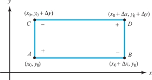
Consider the following expression (see Figure 3.1): \begin{eqnarray*} S(\Delta x, \Delta y) &=&f(x_0+\Delta x,y_0+\Delta y)-f(x_0+\Delta x, y_0)\\ &&-f(x_0,y_0+\Delta y) +f(x_0,y_0). \\[-18pt] \end{eqnarray*}
Holding \(y_0\) and \(\Delta y\) fixed, define \[ g(x)=f(x,y_0+\Delta y)-f(x,y_0), \] so that \(S(\Delta x,\Delta y)=g(x_0+\Delta x)-g(x_0)\), which expresses \(S\) as a difference of differences. By the mean-value theorem for functions of one variable, \(g(x_0+\Delta x)-g(x_0)\) equals \(g'(\bar{x}) \Delta x\) for some \(\bar{x}\) between \(x_0\) and \(x_0+\Delta x\). Hence, \[ S(\Delta x,\Delta y)=\bigg[\frac{\partial f}{\partial x}(\bar{x},y_0+\Delta y)-\frac{\partial f}{\partial x} (\bar{x},y_0)\bigg]\Delta x. \]
152
Applying the mean-value theorem again, there is a \(\bar y\) between \(y_0\) and \(y_0 + \Delta y\) such that \[ S(\Delta x,\Delta y)=\frac{\partial^2\! f}{\partial y\,\partial x}(\bar{x},\bar{y})\,\Delta x\,\Delta y. \]
Because \(\partial^2\! f/\partial y\,\partial x\) is continuous, it follows that \[ \frac{\partial^2\! f}{\partial y\,\partial x}(x_0,y_0)=\mathop{\rm limit}_{(\Delta x,\Delta y)\rightarrow (0,0)}\frac{1}{\Delta x \Delta y}[S(\Delta x,\Delta y)]. \]
Noting that \(S\) is symmetric in \(\Delta x\) and \(\Delta y\), we show in a similar way that \(\partial^2\! f/\partial x\,\partial y\) is given by the same limit formula, which proves the result.
Historical Note
The equality of mixed partial derivatives is one of the most important results of multivariable calculus. It will reappear on several occasions later in the book, when we study vector identities.
In the next historical note, we will discuss the role of partial derivatives in the formulation of many of the basic equations governing physical phenomena. One of the giants in this era was Leonhard Euler (1707–1783), who developed the equations of fluid mechanics that bear his name—the Euler equations. It was in connection with the needs of this development that he discovered, around 1734, the equality of mixed partial derivatives. Euler was about 27 years old at the time.
In Exercise 17 we ask you to deduce from Theorem 1 that for a \(C^3\) function of \(x,y\), and \(z\), \[ \frac{\partial^3\! f}{\partial x\,\partial y\,\partial z}=\frac{\partial^3\! f}{\partial z\,\partial y\,\partial x}=\frac{\partial^3\! f}{\partial y\,\partial z\,\partial x},\qquad\hbox{etc.} \]
In other words, we can compute iterated partial derivatives in any order we please.
example 4
Verify the equality of the mixed second partial derivatives for the function \[ f(x,y)=xe^y+yx^2. \]
solution Here \[ \begin{array}{r@{\,}l@{\qquad}rl } \displaystyle\frac{\partial f}{\partial x} &=e^y+2xy, & \displaystyle\frac{\partial f}{\partial y} &=xe^y+x^2,\\[12pt] \displaystyle\frac{\partial^2\! f}{\partial y\,\partial x} &=e^y+2x, &\displaystyle\frac{\partial^2\! f}{\partial x\,\partial y} &=e^y+2x, \end{array} \] and so we have \[ \frac{\partial^2 \!f}{\partial y\,\partial x}=\frac{\partial^2\! f}{\partial x\, \partial y}. \]
Sometimes the notation \(f_x,f_y,f_z\) is used for the partial derivatives: \(f_x=\partial f/\partial x,\) and so on. With this notation, we write \(f_{xy}={(f_x)}_y\), and so equality of the mixed partials is denoted by \(f_{xy}=f_{yx}\). Notice that \(f_{xy}=\partial^2 \!f/\partial y\,\partial x\), so the order of \(x\) and \(y\) is reversed in the two notations; fortunately, the equality of mixed partials makes this potential ambiguity irrelevant. The following example illustrates this subscript notation.
153
example 5
Let \[ z=f(x,y)=e^x\sin xy \] and write \(x=g(s,t),y=h(s,t)\) for certain functions \(g\) and \(h\). Let \[ k(s,t)=f(g(s,t),h(s,t)). \]
Calculate \(k_{st}\).
solution By the chain rule, \[ k_s=f_xg_s+f_yh_s=(e^x\sin xy +ye^x\cos xy)g_s+(xe^x\cos xy)h_s. \]
Differentiating in \(t\) using the product rules gives \[ k_{st}={(f_x)}_tg_s+f_x{(g_s)}_t+{(f_y)}_th_s+f_y{(h_s)}_t. \]
Applying the chain rule again to \({(f_x)}_t\) and \({(f_y)}_t\) gives \[ {(f_x)}_t=f_{xx}g_t+f_{xy}h_t \quad \hbox{and} \quad {(f_y)}_t=f_{yx}g_t+f_{yy}h_t, \] and so \(k_{st}\) becomes \begin{eqnarray*} k_{st} &=&(f_{xx}g_t+f_{xy}h_t)g_s+f_x g_{st}+(f_{yx}g_t+f_{yy}h_t)h_s+f_yh_{st}\\ &=&f_{xx}g_tg_s+f_{xy}(h_tg_s+h_sg_t)+f_{yy}h_th_s+f_xg_{st}+f_yh_{st}.\\[-19pt] \end{eqnarray*}
Notice that this last formula is symmetric in \((s,t)\), verifying the equality \(k_{st}=k_{ts}\). Computing \(f_{xx},f_{xy}\), and \(f_{yy}\), we get \begin{eqnarray*} k_{st} &=&(e^x\sin xy+2ye^x\cos xy-y^2e^x\sin xy)g_tg_s\\ &&{+}\,(xe^x\cos xy +e^x\cos xy-xy e^x \sin xy)(h_tg_s+h_sg_t)\\ &&{-}\,(x^2e^x\sin xy)h_th_s+(e^x\sin xy +ye^x\cos xy)g_{st}+(xe^x\cos xy)h_{st},\\[-19pt] \end{eqnarray*} in which it is understood that \(x=g(s,t)\) and \(y=h(s,t)\).
Some Partial Differential Equations
Philosophy [nature] is written in that great book which ever is before our eyes—I mean the universe—but we cannot understand it if we do not first learn the language and grasp the symbols in which it is written. The book is written in mathematical language, and the symbols are triangles, circles and other geometrical figures, without whose help it is impossible to comprehend a single word of it; without which one wanders in vain through a dark labyrinth.
—Galileo
Historical Note
This quotation illustrates the Greek belief, again popular in the time of Galileo, that much of nature could be described using mathematics. In the latter part of the seventeenth century this thinking was dramatically reinforced when Newton used his law of gravitation to derive Kepler’s three laws of celestial motion (see Section 4.1) to explain the tides, and to show that the earth was flattened at the poles. The impact of this philosophy on mathematics was substantial, and many mathematicians sought to “mathematize” nature. The extent to which mathematics pervades the physical sciences today (and, to an increasing amount, economics and the social and life sciences) is testament to the success of these endeavors. Correspondingly, the attempts to mathematize nature have often led to new mathematical discoveries.
154
Many of the laws of nature were described in terms of either ordinary differential equations (ODEs, equations involving the derivatives of functions of one variable alone, such as the laws of planetary motion) or partial differential equations (PDEs), that is, equations involving partial derivatives of functions. To give you some historical perspective and offer motivation for studying partial derivatives, we present a brief description of three of the most famous partial differential equations: the heat equation, the potential equation (or Laplace’s equation), and the wave equation. (Further information on some PDEs is given in Section 8.5.)
THE HEAT EQUATION. In the early part of the nineteenth century the French mathematician Joseph Fourier (1768–1830) took up the study of heat. Heat flow had obvious applications to both industrial and scientific problems: A better understanding of it would, for example, make possible more efficient smelting of metals and would enable scientists to determine the temperature of a body given the temperature at its boundary, and to approximate the temperature of the earth’s interior.
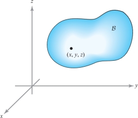
Let a homogeneous body \(\mathcal{B} \subset {\mathbb R}^3\) (Figure 3.2) be represented by some region in 3-space. Let \(T\)(\(x\), \(y\), \(z\), \(t\)) denote the temperature of the body at the point (\(x\), \(y\), \(z\)) at time \(t\). Fourier proved, on the basis of physical principles (described in Section 8.5), that \(T\) must satisfy the partial differential equation called the heat equation, \begin{equation} k\bigg(\frac{\partial^2 T}{\partial x^2}+\frac{\partial^2 T}{\partial y^{\,2}}+\frac{\partial^2 T}{\partial z^{\,2}}\bigg)=\frac{\partial T}{\partial t}\hbox{,} \end{equation} where \(k\) is a constant whose value depends on the conductivity of the material comprising the body.
Fourier used this equation to solve problems in heat conduction. In fact, his investigations into the solutions of equation (1) led him to the discovery of Fourier series.
155
THE POTENTIAL EQUATION. Consider the gravitational potential \(V\) (often called Newton’s potential) of a mass \(m\) at a point (\(x\), \(y\), \(z\)) caused by a point mass \(M\) situated at the origin. This potential is given by \(V=-Gm\,M/r\), where \(r={\textstyle\sqrt{x^2+y^{\,2}+z^{\,2}}}\). The potential \(V\) satisfies the equation \begin{equation} \frac{\partial^2 V}{\partial x^2}+\frac{\partial^2 V}{\partial y^{\,2}}+\frac{\partial^2 V}{\partial z^{\,2}}=0 \end{equation} everywhere except at the origin, as we will check in the next chapter (see also Exercise 25). This equation is known as Laplace’s equation. Pierre-Simon de Laplace (1749–1827) had worked on the gravitational attraction of nonpoint masses and was the first to consider equation (2) with regard to gravitational attraction. He gave arguments (later shown to be incorrect) that equation (2) held for any body and any point whether inside or outside that body. However, Laplace was not the first person to write down equation (2). The potential equation appeared for the first time in one of Euler’s major papers in 1752, “Principles of the Motions of Fluids,” in which he derived the potential equation with regard to the motion of (incompressible) fluids. Euler remarked that he had no idea how to solve equation (2). Poisson later showed that if (\(x\), \(y\), \(z\)) lies inside an attracting body, then \(V\) satisfies the equation \begin{equation} \frac{\partial^2 V}{\partial x^2}+\frac{\partial^2 V}{\partial y^{\,2}}+\frac{\partial^2 V}{\partial z^{\,2}}=-4\pi\rho, \end{equation} where \(\rho\) is the mass density of the attracting body. Equation (3) is now called Poisson’s equation. Poisson was also the first to point out the importance of this equation for problems involving electric fields. Notice that if the temperature \(T\) is constant in time, then the heat equation (1) reduces to Laplace’s equation (2).
Laplace’s and Poisson’s equations are fundamental to many fields besides fluid mechanics, gravitational fields, and electrostatic fields. For example, they are useful for studying soap films and liquid crystals (see The Parsimonious Universe: Shape and Form in the Natural World by S. Hildebrandt and A. Tromba, Springer-Verlag, New York/Berlin, 1995).
THE WAVE EQUATION. The linear wave equation in space has the form \begin{equation} \frac{\partial^2\! f}{\partial x^2}+\frac{\partial^2\! f}{\partial y^{\,2}}+\frac{\partial^2 \! f}{\partial z^{\,2}}=c^{\,\,2}\,\frac{\partial^2 \! f}{\partial t^2}. \end{equation}
The one-dimensional wave equation \begin{equation*} \frac{\partial^2\! f}{\partial x^2}=c^{\,\,2}\,\frac{\partial^2\! f}{\partial t^2}\tag{4'} \end{equation*} was derived in about 1727 by Johann II Bernoulli and several years later by Jean Le Rond d’Alembert in the study of how to determine the motion of a vibrating string (such as a violin string). Equation (4) became useful in the study of both vibrating bodies and elasticity. As we shall see when we consider Maxwell’s equations for electromagnetism in Section 8.5, this equation also arises in the study of the propagation of electromagnetic radiation and sound waves.
156
example 6
As we have pointed out, the heat equation, originating around 1800, is one of the important and classic partial differential equations. It describes the conduction of heat in a solid body. For example, understanding the dissipation of heat is important for industry, as well as for scientists understanding heat stresses on a capsule reentering the earth’s atmosphere.
Consider a thin rod of length \(l\) (Figure 3.3).
We now show that \[ u(x, t)= \frac{1}{t^{1/2}} e^{-x^2/4t} \] is a solution of the heat equation \[ \frac{\partial u}{\partial t} = \frac{\partial^2 u}{\partial x^2}. \]
solution By the chain rule \begin{eqnarray*} \frac{\partial u}{\partial t} &=& -\frac{1}{2t^{3/2}} e^{-x^2/4t} + \frac{1}{t^{1/2}} e^{-x^2/4t} \frac{d}{dt}\Big(\frac{-x^2}{4t}\Big) \\[6pt] &=& -\frac{1}{2t^{3/2}} e^{-x^2/4t} + \frac{1}{t^{1/2}} \cdot \frac{x^2}{4t^2} e^{-x^2/4t} \\[6pt] &=& \frac{1}{2t^{3/2}} \bigg(-1+\frac{x^2}{2t} \bigg) e^{-x^2/4t}, \end{eqnarray*} whereas \begin{eqnarray*} \frac{\partial u}{\partial x} &=& -\frac{x}{2t^{3/2}} e^{-x^2/4t} \\[6pt] \frac{\partial^2 u}{\partial x^2} &=& -\frac{1}{2t^{3/2}} e^{-x^2/4t} + \frac{x^2}{4t} e^{-x^2/4t} \\[3pt] &=& \frac{\partial u}{\partial t}. \end{eqnarray*}
This solution is called a fundamental solution to the heat equation.