5.2 Introduction
This section discusses some geometric aspects of the double integral, deferring a more rigorous discussion in terms of Riemann sums until Section 5.3.
Double Integrals as Volumes
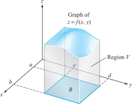
Consider a continuous function of two variables \(f\colon R\subset {\mathbb R}^2\to {\mathbb R}\) whose domain \(R\) is a rectangle with sides parallel to the coordinate axes. The rectangle \(R\) can be described in terms of the two closed intervals \([a, b]\) and \([c, d]\), representing the sides of \(R\) along the \(x\) and \(y\) axes, respectively, as in Figure 5.1. In this case, we say that \(R\) is the Cartesian product of \([a, b]\) and \([c, d]\) and write \(R=[a,b]\times [c,d]\).
Assume that \(f(x,y)\geq 0\) on \(R\), so that the graph of \(z = f(x, y)\) is a surface lying above the rectangle \(R\). This surface, the rectangle \(R\), and the four planes \(x = a, x = b, y =c\), and \(y = d\) form the boundary of a region \(V\) in space (see Figure 5.1).
The problem of how to rigorously define the volume of \(V\) has to be faced, and we shall solve it in Section 5.3 by the classic method of exhaustion, or rather, in more modern terms, the method of Riemann sums. To gain an intuitive grasp of the double integral, we provisionally assume that the volume of a region has been defined.
264
Double Integrals
The volume of the region above \(R\) and under the graph of a nonnegative function \(f\) is called the (double) integral of \(f\) over \(R\) and is denoted by \[ \intop\!\!\!\intop\nolimits_{R}f(x,y)\,{\it dA}, \hbox{or} \intop\!\!\!\intop\nolimits_{R}f(x,y)\,{\it dx} \,{\it dy}. \]
example 1
(a) If \(f\) is defined by \(f(x,y)=k\), where \(k\) is a positive constant, then \[ \intop\!\!\!\intop\nolimits_Rf(x,y)\, {\it dA}= k(b-a)(d-c), \] because the integral is equal to the volume of a rectangular box with base \(R\) and height \(k\).
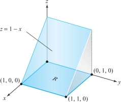
(b) If \(f(x,y)=1-x\) and \(R=[0,1]\times [0,1]\), then \[ \intop\!\!\!\intop\nolimits_R f(x,y)\, {\it dA}=\frac{1}{2}, \] because the integral is equal to the volume of the triangular solid shown in Figure \(5.1.2\).
265
example 2
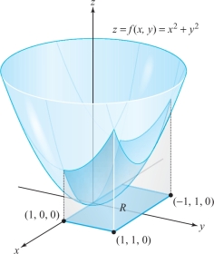
Suppose \(z=f(x,y)=x^2+y^2\) and \(R=[-1,1]\times [0,1]\). Then the integral \({\intop\!\!\!\intop}_R(x^2+y^2)\,{\it dx} \,{\it dy}\) is equal to the volume of the solid sketched in Figure 5.3. We shall compute this integral in Example \(3\).
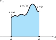
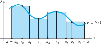
These ideas are similar to those for a single integral \(\int_a^b f(x)\, {\it dx}\), which represents the area under the graph of \(f\) if \(f \ge 0\); see Figure 5.4.footnote #
Single integrals \(\int_a^b f(x)\, {\it dx}\) can be rigorously defined, without recourse to the area concept, as a limit of Riemann sums. The idea is to approximate \(\int_a^b f(x)\, {\it dx}\) by choosing a partition \(a=x_0<x_1<\cdots<x_n=b\) of \([a,b]\), selecting points \(c_i\in [x_i,x_{i+1}]\), and forming the Riemann sum \[ \sum^{n-1}_{i=0}f(c_i)(x_{i+1}-x_i)\approx \int_a^b f(x)\, {\it dx} \] (see Figure 5.5). We examine the analogous process for double integrals in the next section.
Cavalieri’s Principle
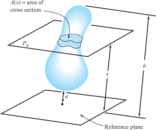
There is a useful method for computing volumes, known as Cavalieri’s principle. Suppose we have a solid body and we let \(A(x)\) denote its cross-sectional area in a plane \(P_x\) measured at a distance \(x\) from a reference plane (Figure 5.6).
266
According to Cavalieri’s principle, the volume of the body is given by \[ \hbox{volume} = \int_a^b A(x)\, {\it dx} , \] where \(a\) and \(b\) are the minimum and maximum distances from the reference plane. This can be made intuitively clear as follows. If we partition \([a,b]\) into \(n\)-equal parts by taking \(a=x_0<x_1<\cdots<x_n=b\), then if \(\Delta x= x_{i + 1} - x_i\) an approximating Riemann sum for the preceding integral is \[ \sum_{i=0}^{n-1}A(c_i)(x_{i+1}-x_i)=\sum_{i=0}^{n-1}A(c_i)\Delta x. \]
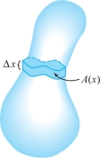
But this sum also approximates the volume of the body, because \(A(x)\, \Delta x\) is the volume of a slab with cross-sectional area \(A(x)\) and thickness \(\Delta x\) (Figure 5.7). Therefore, it is reasonable to accept the preceding formula for the volume. A more careful justification of this method is given in the Internet supplement for Chapter 5.
The Slice Method—Cavalieri’s Principle
Let \(S\) be a solid and, for \(x\) satisfying \(a\leq x\leq b\), let \(P_x\) be a family of parallel planes such that:
- \(S\) lies between \(P_a\) and \(P_b\);
- The area of the slice of \(S\) cut by \(P_x\) is \(A(x)\).
Then the volume of \(S\) is equal to \[ \int_a^bA(x)\,{\it dx}. \]
Historical Note
Bonaventura Cavalieri (1598–1647) was a pupil of Galileo and a professor in Bologna. His investigations into area and volume were important building blocks of the foundations of calculus. Although his methods were criticized by his contemporaries, similar ideas had been used by Archimedes in antiquity and were later taken up by the “fathers” of calculus, Newton and Leibniz.
Reduction to Iterated Integrals
267
We now use Cavalieri’s principle to evaluate double integrals. Consider the solid region under a graph \(z = f(x, y)\) defined on the region \([a,b]\times [c,d]\), where \(f\) is continuous and greater than zero. There are two natural cross-sectional area functions: one obtained by using cutting planes perpendicular to the \(x\) axis, and the other obtained by using cutting planes perpendicular to the \(y\) axis. The cross section determined by a cutting plane \(x = x_0\), of the first sort, is the plane region under the graph of \(z = f(x_0, y)\) from \(y = c\) to \(y = d\) (Figure 5.8).
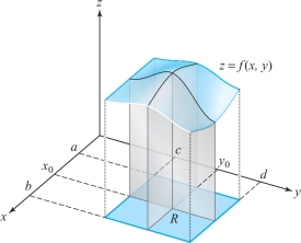
When we fix \(x = x_0\), we obtain the function \(y\mapsto f(x_0,y)\), which is continuous on \([c, d]\). The cross-sectional area \(A(x_0)\) is, therefore, equal to the integral \(\int_c^d f(x_0, y) \,{\it dy}\). Thus, the cross-sectional area function \(A\) has domain \([a, b]\), and is given by the rule \(A\colon x\mapsto \int_c^d f(x,y) \,{\it dy}\). By Cavalieri’s principle, the volume \(V\) of the region under \(z =f(x, y)\) must be equal to \[ V= \int_a^b A(x)\, {\it dx} = \int^b_a \bigg[ \int_c^d f(x,y) \,{\it dy} \bigg]\, {\it dx} . \]
The integral \(\int_a^b\big[\int_c^d f(x,y) \,{\it dy} \big] {\it dx}\) is known as an iterated integral because it is obtained by integrating with respect to \(y\) and then integrating the result with respect to \(x\). Because \({\intop\!\!\!\intop}_R f(x,y)\, {\it dA}\) is equal to the volume \(V\), we get the following result.
Double and Iterated Integrals
\begin{equation} \intop\!\!\!\intop\nolimits_{R} f(x,y)\, {\it dA} = \int_a^b \bigg[ \int_c^d f(x,y)\, {\it dy} \bigg]\, {\it dx} \end{equation}
If we use cutting planes perpendicular to the \(y\) axis, we obtain \begin{equation} \intop\!\!\!\intop\nolimits_{R} f(x,y)\, {\it dA} = \int_c^d \bigg[ \int_a^b f(x,y)\, {\it dx} \bigg]\, {\it dy} \end{equation}
The expression on the right of formula (2) is the iterated integral obtained by integrating with respect to \(x\) and then integrating the result with respect to \(y\).
268
Thus, if our intuition about volumes is correct, formulas (1) and (2) ought to be valid. This is in fact true when the concepts we are discussing are defined rigorously, and is known as Fubini’s theorem. We give a proof of this theorem in the next section.
As the following examples illustrate, the notion of the iterated integral and equations (1) and (2) provide a powerful method for computing the double integral of a function of two variables.
example 3
Evaluate the integral \[ \intop\!\!\!\intop\nolimits_{R}\,(x^2+y^2)\, {\it dx} \,{\it dy}, \] where \(R=[-1,1]\times [0,1]\).
solution By equation (2), \[ \intop\!\!\!\intop\nolimits_{R} \, (x^2+y^2)\, {\it dx} \,{\it dy} = \int_0^1 \bigg[ \int_{-1}^1\, (x^2+y^2)\, {\it dx} \bigg]\,{\it dy}. \]
To find \(\int_{-1}^1\, (x^2+y^2)\, {\it dx}\), we treat \(y\) as a constant and integrate with respect to \(x\). Because \(x^3/3+y^2x\) is an antiderivative of \(x^2+y^2\) with respect to \(x\), we can integrate, using the fundamental theorem of calculus, to obtain \[ \int_{-1}^1(x^2+y^2)\, {\it dx} = \bigg[\frac{x^3}{3}+y^2x\bigg]_{x=-1}^1=\frac{2}{3}+2y^2 . \]
Next, we integrate \(\frac{2}{3}+2y^2\) with respect to \(y\) from 0 to 1 to obtain \[ \int_0^1 \bigg( \frac{2}{3} \,+\,2y^2\bigg) \,{\it dy}=\bigg[ \frac{2}{3} y\,+\, \frac{2}{3} y^3\bigg]^1_{y=0}= \frac{4}{3}. \]
Hence, the volume of the solid we saw in Figure 5.3 is \(4/3\).
For completeness, let us evaluate \({\intop\!\!\!\intop}_R(x^2+y^2)\, {\it dx} \,{\it dy}\) using equation (1)—that is, integrating with respect to \(y\) first and then with respect to \(x\). We have \[ \intop\!\!\!\intop\nolimits_{R} \, (x^2+y^2)\, {\it dx} \,{\it dy} = \int_{-1}^1 \bigg[ \int_0^1 (x^2+y^2) \,{\it dy} \bigg]{\it dx}. \]
Treating \(x\) as a constant in the \(y\) integration, we obtain \[ \int^1_0(x^2+y^2) \,{\it dy} =\bigg[x^2y+\frac{y^3}{3}\bigg]_{y=0}^1=x^2+\frac{1}{3}. \]
Next, we evaluate \(\int_{-1}^1\big(x^2+\frac{1}{3}\big)\, {\it dx} \,\) to obtain \[ \int_{-1}^1\bigg(x^2+\frac{1}{3}\bigg)\, {\it dx} =\bigg[\frac{x^3}{3}+\frac{x}{3} \bigg]_{x=-1}^1=\frac{4}{3}, \] which agrees with our previous answer.
269
example 4
Compute the double integral \({\intop\!\!\!\intop}_{S}\cos x \sin y\, {\it dx} \,{\it dy} \), where \(S\) is the square \([0,\pi/2] \times [0, \pi/2]\) (see Figure 5.9).
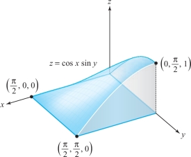
solution By equation (2), \begin{eqnarray*} \intop\!\!\!\intop\nolimits_{S} \cos x\sin y\, {\it dx} \,{\it dy} &=& \int_0^{\pi/2} \bigg[ \int_0^{\pi/2} \cos x\sin y\, {\it dx} \bigg]{\it dy}\\[4pt] &=& \int_0^{\pi/2}\sin y\bigg[ \int_0^{\pi/2 }\cos x\, {\it dx} \bigg]{\it dy}= \int_0^{\pi/2} \sin y\, {\it dy} =1.\\[-30pt] \end{eqnarray*}
In the next section, we shall use Riemann sums to rigorously define the double integral for a large class of functions of two variables without recourse to the notion of volume. Although we shall drop the requirement that \(f(x,y)\geq 0\), equations (1) and (2) will remain valid. Therefore, the iterated integral will again provide the key to computing the double integral. In Section 5.4, we treat double integrals over regions more general than rectangles.
Finally, we remark that it is common to delete the brackets in iterated integrals such as equations (1) and (2) and to write \[ \int_a^b \int_c^d f(x,y)\, {\it dy}\, {\it dx}\qquad \hbox{in place of} \int_a^b \bigg[ \int_c^df(x,y)\, {\it dy} \bigg]\, {\it dx} \] and \[ \int_c^d \int_a^bf(x,y)\, {\it dx}\, {\it dy}\qquad \hbox{in place of} \int_c^d\bigg[ \int_a^bf(x,y)\, {\it dx} \bigg]\, {\it dy}. \]