6.2 The Geometry of Maps from ℝ² to ℝ²
In this section, we shall be interested in maps from subsets of \({\mathbb R}^2\) to \({\mathbb R}^2\). The resulting geometric understanding will be useful in the next section, when we discuss the change of variables formula for multiple integrals.
Maps of One Region to Another
Let \(D^*\) be a subset of \({\mathbb R}^2\); suppose we consider a continuously differentiable map \(T \colon D^* \to {\mathbb R}^2\), so \(T\) takes points in \(D^*\) to points in \({\mathbb R}^2\). We denote the set of image points by \(D\) or by \(T (D^*)\); hence, \(D = T ( D^*)\) is the set of all points \((x,y) \in {\mathbb R}^2\) such that \[ (x,y) = T (x^*, y^*) \qquad \hbox{for some} \qquad (x^*, y^*) \in D^*. \]
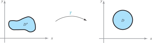
One way to understand the geometry of a map \(T\) is to see how it deforms or changes \(D^*\). For example, Figure 6.1 illustrates a map \(T\) that takes a slightly twisted region into a disk.
example 1
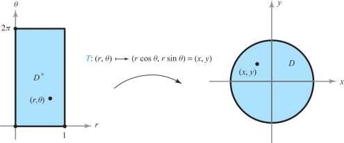
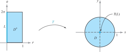
Let \(D^* \subset {\mathbb R}^2\) be the rectangle \(D^* = [0,1] \times [0,2 \pi]\). Then all points in \(D^*\) are of the form \((r, \theta)\), where \(0 \le r \le 1, 0 \le \theta \le 2 \pi\). Let \(T\) be the polar coordinate “change of variables” defined by \(T (r, \theta) = ( r \cos \theta, r \sin \theta)\). Find the image set \(D\).
solution Let \((x,y) = ( r \cos \theta, r \sin \theta)\). Because of the identity \(x^2 + y^2 = r^2 \cos^2 \theta + r^2 \sin^2 \theta = r^2 \le 1\), we see that the set of points \((x,y) \in {\mathbb R}^2\) such that \((x,y) \in D\) has the property that \(x^2 + y^2 \le 1\), and so \(D\) is contained in the unit disk. In addition, any point \((x,y)\) in the unit disk can be written as \((r \cos \theta , r \sin \theta)\) for some \(0 \le r \le 1\) and \(0 \le \theta \le 2 \pi\). Thus, \(D\) is the unit disk (see Figure 6.2).
309
example 2
Let \(T\) be defined by \(T (x,y) = (( x+ y) /2, (x-y) /2)\) and let \(D^* = [-1,1] \times [-1,1] \subset {\mathbb R}^2\) be a square with side of length 2 centered at the origin. Determine the image \(D\) obtained by applying \(T\) to \(D^*\).
solution Let us first determine the effect of \(T\) on the line \({\bf c}_1 (t) = (t,1)\), where \(-1 \le t \le 1\) (see Figure 6.3). We have \(T ( {\bf c}_1 (t))= ( ( t+1)/2, (t-1) /2)\). The map \(t \mapsto T ( {\bf c}_1 (t))\) is a parametrization of the line \(y=x-1, 0 \le x \le 1\), because \((t-1) / 2 = (t+1)/2 -1\). This is the straight line segment joining \((1,0)\) and \((0,-1)\).
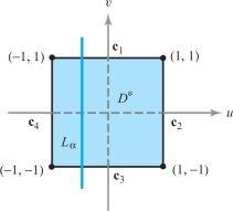
Let \[ \begin{array}{l@{\qquad}l} {\bf c}_2 (t) = (1,t), & -1 \le t \le 1 \\[6pt] {\bf c}_3 (t) = (t, -1), & -1 \le t \le 1 \\[6pt] {\bf c}_4 (t) = (-1,t), & -1 \le t \le 1 \end{array} \] be parametrizations of the other edges of the square \(D^*\). Using the same argument as before, we see that \(T \circ {\bf c}_2\) is a parametrization of the line \(y= 1-x, 0 \le x \le 1\) [the straight line segment joining \((0,1)\) and \((1,0)\)]; \(T \circ {\bf c}_3\) is the line \(y=x+1, -1 \le x \le 0\) joining \((0,1)\) and \(({-}1,0)\); and \(T \circ {\bf c}_4\) is the line \(y = - x-1, -1 \le x \le 0\) joining \(({-}1,0)\) and \((0,{-}1)\). By this time it seems reasonable to guess that \(T\) “flips” the square \(D^*\) over and takes it to the square \(D\) whose vertices are \((1,0), (0,1), (-1,0), (0,-1)\) (Figure 6.4).
310
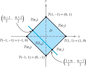
To prove that this is indeed the case, let \(-1 \le \alpha \le 1\) and let \(L_\alpha\) (Figure 6.3) be a fixed line parametrized by \({\bf c} (t) = ( \alpha, t), -1 \le t \le 1\); then \(T ( {\bf c} (t)) = (( \alpha \,{+}\, t) /2, (\alpha \,{-}\,t) /2)\) is a parametrization of the line \(y=-x \,{+}\, \alpha, (\alpha \,{-}\,1) /2 \le x \le (\alpha \,{+}\,1) /2\). This line begins, for \(t\,{=}\,-1\), at the point \(((\alpha \,{-}\,1)/2, (1\,{+}\, \alpha)/2)\) and ends at the point \(((1\,{+}\, \alpha) /2, ( \alpha \,{-}\,1) /2)\); as is easily checked, these points lie on the lines \(T \circ {\bf c}_3\) and \(T \circ {\bf c}_1\), respectively. Thus, as \(\alpha\) varies between \(-1\) and \(1\), \(L_\alpha\) sweeps out the square \(D^*\) while \(T ( L_\alpha)\) sweeps out the square \(D\) determined by the vertices \((-1,0), (0,1), (1,0),\) and \((0,-1)\).
Images of Maps
The following theorem is a useful way to describe the image \(T(D^*)\).
Theorem 1
Let \(A\) be a \(2 \times 2\) matrix with det \(A \ne 0\) and let \(T\) be the linear mapping of \({\mathbb R}^2\) to \({\mathbb R}^2\) given by \(T ({\bf x})= A{\bf x}\) \((\)matrix multiplication\().\) Then \(T\) transforms parallelograms into parallelograms and vertices into vertices\(.\) Moreover, if \(T (D^*)\) is a parallelogram, \(D^*\) must be a parallelogram.
The proof of Theorem 1 is left as Exercises 14 and 16 at the end of this section. This theorem simplifies the result of Example 2, because we need only find the vertices of \(T ( D^*)\) and then connect them by straight lines.
One-to-One Maps
Although we cannot visualize the graph of a function \(T\colon\, {\mathbb R}^2 \to {\mathbb R}^2 \), it does help to consider how the function deforms subsets. However, simply looking at these deformations does not give us a complete picture of the behavior of \(T\). We may characterize \(T\) further by using the notion of a one-to-one correspondence.
Definition
A mapping \(T\) is one-to-one on \(D^*\) if for \((u,v)\) and \((u',v') \in D^*\), \(T (u,v)\) \(=\) \(T (u', v')\) implies that \(u=u'\) and \(v=v'\).
This statement means that two different points of \(D^*\) are not sent into the same point of \(D\) by \(T\). For example, the function \(T (x,y) = (x^2 + y^2 , y^4)\) is not one-to-one, because \(T (1,-1) = (2,1) = T (1,1)\), and yet \((1,-1) \ne (1,1)\).
311
example 3
Consider the polar coordinate mapping function \(T \colon\, {\mathbb R}^2 \to {\mathbb R}^2\) described in Example 1, defined by \(T (r, \theta)= ( r \cos \theta, r \sin \theta)\). Show that \(T\) is not one-to-one if its domain is all of \({\mathbb R}^2\).
solution If \(\theta_1\ne \theta_2\), then \(T (0,\theta_1) = T (0, \theta_2)\), and so \(T\) cannot be one-to-one. This observation implies that if \(L\) is the side of the rectangle \(D^* = [0,1] \times [0, 2 \pi]\) where \(0 \le \theta \le 2 \pi\) and \(r=0\) (Figure 6.5), then \(T\) maps all of \(L\) into a single point, the center of the unit disk \(D\). However, if we consider the set \(S^* = (0,1] \times [0, 2 \pi)\), then \(T \colon\, S^* \to S\) is one-to-one (see Exercise 5). Evidently, in determining whether a function is one-to-one, the domain chosen must be carefully considered.
example 4
Show that the function \(T \colon\, {\mathbb R}^2 \to {\mathbb R}^2\) of Example 2 is one-to-one.
solution Suppose \(T (x,y) = T (x', y')\); then \[ \left( \frac{x+y}{2}, \frac{x-y}{2} \right) = \left( \frac{x^\prime+ y'}{2}, \frac{x' - y'}{2} \right) \] and we have \begin{eqnarray*} x+ y &=& x' + y' ,\\ x - y &=& x' - y' .\\[-17pt] \end{eqnarray*}
Adding, we have \[ 2x =2x'. \]
Thus, \(x = x'\) and, similarly, subtracting gives \(y=y'\), which shows that \(T\) is one-to-one (with domain all of \({\mathbb R}^2\)). Actually, because \(T\) is linear and \(T ( {\bf x}) = A {\bf x}\), where \(A\) is a \(2 \times 2\) matrix, it would also suffice to show that det \(A \ne 0\) (see Exercise 12).
Onto Maps
In Examples 1 and 2, we have been determining the image \(D = T (D^*)\) of a region \(D^*\) under a mapping \(T\). What will be of interest to us in the next section is, in part, the inverse problem: Namely, given \(D\) and a one-to-one mapping \(T\) of \({\mathbb R}^2\) to \({\mathbb R}^2\), find \(D^*\) such that \(T (D^*) =D\).
312
Before we examine this question in more detail, we introduce the notion of “onto.”
Definition
The mapping \(T\) is onto \(D\) if for every point \((x,y) \in D\) there exists at least one point \((u,v)\) in the domain of \(T\) such that \(T (u,v) = (x,y)\).
Thus, if \(T\) is onto, we can solve the equation \(T (u,v) = (x,y)\) for \((u,v)\), given \((x,y) \in D\). If \(T\) is, in addition, one-to-one, this solution is unique. For linear mappings \(T\) of \({\mathbb R}^2\) to \({\mathbb R}^2\) (or \({\mathbb R}^n\) to \({\mathbb R}^n\)) it turns out that one-to-one and onto are equivalent notions (see Exercises 12 and 13).
If we are given a region \(D\) and a mapping \(T\), the determination of a region \(D^*\) such that \(T (D^*) =D\) will be possible only when for every \((x,y) \in D\) there is a \((u,v)\) in the domain of \(T\) such that \(T (u,v) = (x,y)\) (that is, \(T\) must be onto \(D\)). The next example shows that this cannot always be done.
example 5
Let \(T \colon\, {\mathbb R}^2 \to {\mathbb R}^2\) be given by \(T (u,v) = (u,0)\). Let \(D\) be the square, \(D= [0,1] \times [0,1].\) Because \(T\) takes all of \({\mathbb R}^2\) to one axis, it is impossible to find a \(D^*\) such that \(T ( D^*) =D\).
Let us revisit Example 2 using these methods.
example 6
Let \(T\) be defined as in Example 2 and let \(D\) be the square whose vertices are \((1,0),(0,1), (-1,0),(0,-1)\). Find a \(D^*\) with \(T ( D^*) =D\).
solution Because \(T\) is linear and \(T ( {\bf x}) = A {\bf x}\), where \(A\) is a \(2 \times 2\) matrix satisfying det \(A \ne 0\), we know that \(T \colon\, {\mathbb R}^2 \to {\mathbb R}^2\) is onto (see Exercises 12 and 13), and thus \(D^*\) can be found. By Theorem 1, \(D^*\) must be a parallelogram. In order to find \(D^*\), it suffices to find the four points that are mapped onto vertices of \(D\); then, by connecting these points, we will have found \(D^*\). For the vertex \((1, 0)\) of \(D\), we must solve \(T (x,y) = (1,0)= ((x+y) /2, (x-y)/2)\), so that \((x+y)/2 =1, (x-y) /2 =0\). Thus, \((x,y) = (1,1)\) is a vertex of \(D^*\). Solving for the other vertices, we find that \(D^* = [-1,1] \times [-1,1]\). This is in agreement with what we found more laboriously in Example 2.
example 7
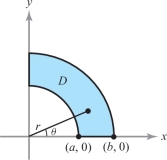
Let \(D\) be the region in the first quadrant lying between the arcs of the circles \(x^2 + y^2 = a^2 , x^2 + y^2 = b^2 , 0 < a < b\) \((\)see Figure 6.6). These circles have equations \(r=a\) and \(r=b\) in polar coordinates. Let \(T\) be the polar-coordinate transformation given by \(T ( r, \theta) = (r \cos \theta, r \sin \theta) = (x,y)\). Find \(D^*\) such that \(T ( D^*) = D\).
solution In the region \(D, a^2 \le x^2 + y^2 \le b^2\); and because \(r^2 = x^2 + y^2\), we see that \(a \le r \le b\). Clearly, for this region \(\theta\) varies between \(0 \le \theta \le \pi /2\). Thus, if \(D^* = [a,b] \times [0, \pi /2]\), we have \(T ( D^*) = D\) and \(T\) is one-to-one.
remark
The inverse function theorem discussed in Section 3.5 is relevant to the material here. It states that if the determinant of \({\bf D} T ( u_0, v_0)\) [which is the matrix of partial derivatives of \(T\) evaluated at \((u_0, v_0)\)] is not zero, then for \((u, v)\) near \((u_0, v_0)\) and \((x,y)\) near \((x_0, y_0) = T (u_0, v_0)\), the equation \(T (u, v) = (x,y)\) can be uniquely solved for \((u, v)\) as functions of \((x,y)\). In particular, by uniqueness, \(T\) is one-to-one near \((u_0, v_0)\); also, \(T\) is onto a neighborhood of \((x_0, y_0)\), because \(T (u,v) = (x,y)\) is solvable for \((u,v)\) if \((x,y)\) is near \((x_0, y_0)\).
313
However, even if \(T\) is one-to-one near every point, and also onto, \(T\) need not be globally one-to-one. Thus, we must exercise caution (see Exercise 17).
Surprisingly, if \(D^*\) and \(D\) are elementary regions and \(T \colon\, D^* \to D\) has the property that the determinant of \({\bf D} T (u, v)\) is not zero for any \((u, v)\) in \(D^*\), and if \(T\) maps the boundary of \(D^*\) in a one-to-one and onto manner to the boundary of \(D\), then \(T\) is one-to-one and onto from \(D^*\) to \(D\). (This proof is beyond the scope of this text.)
In summary, we have:
One-to-One and Onto Mappings
A mapping \(T{:}\, D^{*}\to D\) is one-to-one when it maps distinct points to distinct points. It is onto when the image of \(D^*\) under \(T\) is all of \(D\).
A linear transformation of \({\mathbb R}^n\) to \({\mathbb R}^n\) given by multiplication by a matrix \(A\) is one-to-one and onto when and only when det \(A\neq 0\).