7.5 Area of a Surface
Before proceeding to general surface integrals, let us first consider the problem of computing the area of a surface, just as we considered the problem of finding the arc length of a curve before discussing path integrals.
Definition of Surface Area
384
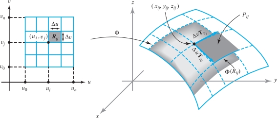
In Section 7.4 we defined a parametrized surface \(S\) to be the image of a function \({\Phi}\colon\, D\subset {\mathbb R}^2\to {\mathbb R}^3\), written as \({\Phi}(u,v)=(x(u,v),y(u,v),z(u,v))\). The map \({\Phi}\) was called the parametrization of \(S\) and \(S\) was said to be regular at \({\Phi}(u,v)\in S\) provided that \({\bf T}_u\times {\bf T}_v\neq {\bf 0}\), where \[ {\bf T}_u=\frac{\partial x}{\partial u}(u,v){\bf i}+ \frac{\partial y}{\partial u}(u,v){\bf j}+ \frac{\partial z}{\partial u}(u,v){\bf k} \] and \[ {\bf T}_v=\frac{\partial x}{\partial v}(u,v){\bf i}+ \frac{\partial y}{\partial v}(u,v){\bf j}+ \frac{\partial z}{\partial v}(u,v){\bf k} . \]
Recall that a regular surface (loosely speaking) is one that has no corners or breaks.
In the rest of this chapter and in the next one, we shall consider only piecewise regular surfaces that are unions of images of parametrized surfaces \({\Phi}_i\colon\, D_i\to {\mathbb R}^3\) for which:
- (i) \(D_i\) is an elementary region in the plane;
- (ii) \({\Phi}_i\) is of class \(C^1\) and one-to-one, except possibly on the boundary of \(D_i \); and
- (iii) \(S_i\), the image of \({\Phi}_i\), is regular, except possibly at a finite number of points.
Definition: Area of a Parametrized Surface
We define the surface areafootnote # \(A(S)\) of a parametrized surface by \begin{equation*} A(S)=\int\!\!\!\int\nolimits_{D}\|{\bf T}_u\times {\bf T}_v\|\,du\,dv,\tag{1} \end{equation*} where \(\|{\bf T}_u \times {\bf T}_v\|\) is the norm of \({\bf T}_u\times {\bf T}_v\). If \(S\) is a union of surfaces \(S_i\), its area is the sum of the areas of the \(S_i\).
As you can easily verify, we have \begin{equation*} \|{\bf T}_u\times {\bf T}_v\|=\sqrt{\bigg[\frac{\partial (x,y)}{\partial (u,v)}\bigg]^2+\bigg[\frac{\partial (y,z)}{\partial (u,v)}\bigg]^2+\bigg[\frac{\partial (x,z)}{\partial (u,v)}\bigg]^2},\tag{2} \end{equation*} where \[ \frac{\partial (x,y)}{\partial (u,v)}=\left| \begin{array}{c@{\quad}c} \displaystyle \frac{\partial x}{\partial u}&\displaystyle \frac{\partial x}{\partial v}\\[9pt] \displaystyle \frac{\partial y}{\partial u}&\displaystyle \frac{\partial y}{\partial v}\\ \end{array}\right|, \] and so on. Thus, formula (1) becomes \begin{equation*} A(S)=\int\!\!\!\int\nolimits_{D}\sqrt{\bigg[\frac{\partial (x,y)}{\partial (u,v)}\bigg]^2+\bigg[\frac{\partial (y,z)}{\partial (u,v)}\bigg]^2+\bigg[\frac{\partial (x,z)}{\partial (u,v)}\bigg]^2} \,du \,dv.\tag{3} \end{equation*}
Justification of the Area Formula
385
We can justify the definition of surface area by analyzing the integral \({\int\!\!\!\int}_D\|{\bf T}_u\times {\bf T}_v\| \,du \,dv\) in terms of Riemann sums. For simplicity, suppose \(D\) is a rectangle; consider the \(n \)th regular partition of \(D\), and let \(R_{\it ij}\) be the \(ij \)th rectangle in the partition, with vertices \((u_i, v_j),(u_{i+1},v_j),(u_i,v_{j+1})\), and \((u_{i+1},v_{j+1}),0\leq i\leq n-1, 0\leq j\leq n-1\). Denote the values of \({\bf T}_u\) and \({\bf T}_v\) at \((u_i,v_j)\) by \({\bf T}_{u_i}\) and \({\bf T}_{v_j}\). We can think of the vectors \({ \Delta} u{\bf T}_{u_i}\) and \( { \Delta} v{\bf T}_{v_j}\) as tangent to the surface at \({\Phi}(u_i,v_j)=(x_{\it ij},y_{\it ij},z_{\it ij})\), where \( { \Delta} u=u_{i+1}-u_i, { \Delta} v=v_{j+1}-v_j\). Then these vectors form a parallelogram \(P_{\it ij}\) that lies in the plane tangent to the surface at \((x_{\it ij},y_{\it ij},z_{\it ij})\) (see Figure 7.30). We thus have a “patchwork cover” of the surface by the \(P_{\it ij}\). For \(n\) large, the area of \(P_{\it ij}\) is a good approximation to the area of \({\Phi}(R_{\it ij})\). Because the area of the parallelogram spanned by two vectors \({\bf v}_1\) and \({\bf v}_2\) is \(\|{\bf v}_1\times {\bf v}_2\|\) (see Chapter 1), we see that \[ A(P_{\it ij})=\| { \Delta} u {\bf T}_{u_i}\times { \Delta} v{\bf T}_{v_j}\| =\|{\bf T}_{u_i}\times {\bf T}_{v_j}\| { \Delta} u\, { \Delta} v. \]
Therefore, the area of the patchwork cover is \[ A_n=\sum_{i=0}^{n-1}\sum^{n-1}_{j=0}A(P_{\it ij})= \sum_{i=0}^{n-1}\sum^{n-1}_{j=0}\|{\bf T}_{u_i}\times {\bf T}_{v_j}\|\, { \Delta} u \,{ \Delta} v. \]
As \(n \to \infty\), the sums \(A_n\) converge to the integral \[ \int\!\!\!\int\nolimits_{D} \|{\bf T}_{u}\times {\bf T}_{v}\| \,du \,dv. \]
Because \(A_n\) should approximate the surface area better and better as \(n \to \infty\), we are led to formula (1) as a reasonable definition of \(A(S)\).
example 1
Let \(D\) be the region determined by \(0\leq \theta \leq 2\pi ,0\leq r\leq 1\) and let the function \({\Phi}\colon\, D\to {\mathbb R}^3\), defined by \[ x=r\cos \theta,\qquad y=r \sin \theta ,\qquad z=r, \] be a parametrization of a cone \({S}\) (see Figure 7.29). Find its surface area.
386
solution In formula (3), \begin{eqnarray*} \frac{\partial (x,y)}{\partial (r,\theta)}&=&\Big| \begin{array}{cr} \cos \theta & -r \sin \theta \\ \sin \theta & r \cos \theta \end{array}\Big|=r,\\[5pt] \frac{\partial (y,z)}{\partial (r,\theta)}&=&\Big| \begin{array}{c@{\qquad}c} \sin\theta & r \cos\theta \\ 1 & 0 \end{array}\Big|=-r \cos \theta,\\[-15pt] \end{eqnarray*} and \[ \frac{\partial (x,z)}{\partial (r,\theta)}=\Big| \begin{array}{cc} \cos\theta & -r \sin\theta \\ 1 & 0 \end{array}\Big|=r \sin \theta, \] so the area integrand is \[ \|{\bf T}_r\times {\bf T}_{\theta}\|= \sqrt{r^2+r^2\cos^2\theta +r^2 \sin^2\theta}=r\sqrt{2}. \]
Clearly, \(\|{\bf T}_r\times {\bf T}_{\theta}\|\) vanishes for \(r = 0\), but \({\Phi}(0,\theta)=(0,0,0)\) for any \(\theta\). Thus, \((0, 0, 0)\) is the only point where the surface is not regular. We have \[ \int\!\!\!\int\nolimits_{D}\|{\bf T}_r\times {\bf T}_{\theta}\|\,dr \,d\theta = \int^{2\pi}_0\int^1_0 \sqrt{2}r \,dr \,d\theta = \int^{2\pi}_0\frac{1}{2}\sqrt{2} \,d\theta =\sqrt{2}\pi. \]
To confirm that this is the area of \({\Phi}(D)\), we must verify that \({\Phi}\) is one-to-one (for points not on the boundary of \(D \)). Let \(D^0\) be the set of \((r,\theta)\) with \(0<r<1\) and \(0<\theta <2\pi\). Hence, \(D^0\) is \(D\) without its boundary. To see that \({\Phi}\colon\, D^0 \to {\mathbb R}^3\) is one-to-one, assume that \({\Phi}(r,\theta)={\Phi}(r',\theta')\) for \((r,\theta)\) and \((r',\theta')\in D^0\). Then \[ r\cos \theta=r'\cos \theta',\qquad r\sin \theta =r'\sin \theta', \qquad r=r'. \]
From these equations it follows that \(\cos \theta =\cos \theta'\) and \(\sin \theta=\sin \theta'\). Thus, either \(\theta=\theta'\) or \(\theta =\theta'+2\pi n\). But the second case is impossible for \(n\) a nonzero integer, because both \(\theta\) and \(\theta'\) belong to the open interval \((0,2\pi)\) and thus cannot be more than \(2\pi\) radians apart. This proves that off the boundary, \({\Phi}\) is one-to-one. (Is \({\Phi}\colon\, D \to {\mathbb R}^3\) one-to-one?) In future examples, we shall not usually verify that the parametrization is one-to-one when it is intuitively clear.
example 2
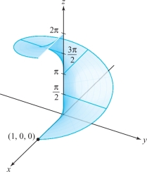
A helicoid is defined by \({\Phi}\colon\, D\to {\mathbb R}^3\), where \[ x=r\cos \theta,\qquad y=r\sin \theta ,\qquad z=\theta \] and \(D\) is the region where \(0 \leq \theta \leq 2\pi\) and \(0\leq r\leq 1\) (Figure 7.31). Find its area.
387
solution We compute \(\partial (x,y)/\partial (r,\theta)=r\) as in Example 1, and \begin{eqnarray*} \frac{\partial (y,z)}{\partial (r,\theta)}&=&\Big| \begin{array}{c@{\quad}c} \sin\theta& r\cos \theta\\ 0&1 \end{array}\Big|=\sin \theta,\\[4pt] \frac{\partial (x,z)}{\partial (r,\theta)}&=&\Big| \begin{array}{c@{\quad}c} \cos\theta& -r\sin \theta\\ 0&1 \end{array}\Big|=\cos \theta. \end{eqnarray*}
The area integrand is therefore \(\sqrt{r^2+1}\), which never vanishes, so the surface is regular. The area of the helicoid is \[ \int\!\!\!\int\nolimits_{D}\|{\bf T}_r\times {\bf T}_{\theta} \| \,dr \,d\theta= \int^{2\pi}_0\int^1_0\sqrt{r^2+1}\,dr\, d\theta =2\pi \int^1_0\sqrt{r^2+1}\,dr. \]
After a little computation (using the table of integrals), we find that this integral is equal to \[ \pi[\sqrt{2}+\log\,(1+\sqrt{2})]. \]
Surface Area of a Graph
A surface \(S\) given in the form \(z \,{=}\, g(x, y)\), where \((x,y)\,{\in}\, D\), admits the parametri- zation \[ x=u,\qquad y=v,\qquad z=g(u, v) \] for \((u,v)\in D\). When \(g\) is of class \(C^1\), this parametrization is smooth, and the formula for surface area reduces to \begin{equation*} A(S)=\int\!\!\!\int\nolimits_{D} \left(\sqrt{\bigg(\frac{\partial g}{\partial x}\bigg)^2+ \bigg(\frac{\partial g}{\partial y}\bigg)^2+1 }\,\right){\it dA},\tag{4} \end{equation*} after applying the formulas \[ {\bf T}_u={\bf i} + \frac{\partial g}{\partial u}{\bf k}, \qquad {\bf T}_v={\bf j} + \frac{\partial g}{\partial v}{\bf k}, \] and \[ {\bf T}_u\times {\bf T}_v=-\frac{\partial g}{\partial u}{\bf i} -\frac{\partial g}{\partial v}{\bf j}+{\bf k}=-\frac{\partial g} {\partial x}{\bf i}- \frac{\partial g}{\partial y}{\bf j}+{\bf k}, \] as noted in Example 4 of Section 7.4.
Surfaces of Revolution
In most books on one-variable calculus, it is shown that the lateral surface area generated by revolving the graph of a function \(y = f(x)\) about the \(x\) axis is given by \begin{equation*} A = 2\pi\int^b_a (|f(x)|{\textstyle\sqrt{1+[f'(x)]^2}} )\,{\it dx}.\tag{5} \end{equation*}
388
If the graph is revolved about the \(y\) axis, the surface area is \begin{equation*} A = 2\pi\int^b_a (|x| {\textstyle\sqrt{1+[f'(x)]^2}})\,{\it dx}.\tag{6} \end{equation*}
We shall derive formula (5) by using the methods just developed; we can obtain formula (6) in a similar fashion (Exercise 10).
To derive formula (5) from formula (3), we must give a parametrization of \(S\). Define the parametrization by \[ x=u,\qquad y=f(u)\cos v,\qquad z=f(u)\sin v \] over the region \(D\) given by \[ a\leq u\leq b,\qquad 0\leq v\leq 2\pi. \]
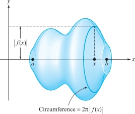
This is indeed a parametrization of \(S\), because for fixed \(u\), the point \[ (u,f(u)\cos v,f(u)\sin v) \] traces out a circle of radius \(|f(u)|\) with the center \((u, 0, 0)\) (Figure 7.32).
We calculate \[ \frac{\partial (x,y)}{\partial (u,v)}=-f(u)\sin v,\qquad \frac{\partial (y,z)}{\partial (u,v)}=f(u)f'(u),\qquad \frac{\partial (x,z)}{\partial (u,v)}=f(u)\cos v, \] and so by formula (3) \begin{eqnarray*} A(S)&=& \int\!\!\!\int\nolimits_{D}{\textstyle\sqrt{\bigg[{\displaystyle\frac{\partial (x,y)}{\partial (u,v)}}\bigg]^2+\bigg[{\displaystyle\frac{\partial (y,z)}{\partial (u,v)}}\bigg]^2+\bigg[{\displaystyle\frac{\partial (x,z)}{\partial (u,v)}}\bigg]^2}}du\,dv\\[5pt] &=&\int\!\!\!\int\nolimits_{D} {\textstyle\sqrt{[f(u)]^2\sin^2 v+ [f(u)]^2[f'(u)]^2+[f(u)]^2 \cos^2 v }}\,du \,dv\\[5pt] &=&\int\!\!\!\int\nolimits_{D}|f(u)|{\textstyle\sqrt{1+[f'(u)]^2}}\,du \,dv\\[5pt] &=&\int^b_a\int^{2\pi}_0 |f(u)|{\textstyle\sqrt{1+[f'(u)]^2}} \,dv \,du\\[4pt] &=&2\pi\int^b_a|f(u)| {\textstyle\sqrt{1+[f'(u)]^2}} \,du, \end{eqnarray*} which is formula (5).
389
If \(S\) is the surface of revolution, then \(2\pi|f(x)|\) is the circumference of the vertical cross section to \(S\) at the point \(x\) (Figure 7.32). Observe that we can write \[ 2\pi \int^b_a|f(x)|{\textstyle\sqrt{1+[f'(x)]^2}} \,{\it dx} =\int_{\bf c} 2 \pi |f(x)| \,{\it ds} , \] where the expression on the right is the path integral of \(2\pi|f(x)|\) along the path given by \({\bf c}\colon\, [a,b]\to {\mathbb R}^2,t\mapsto (t,f(t))\). Therefore, the lateral surface of a solid of revolution is obtained by integrating the cross-sectional circumference along the path that is the graph of the given function.
Historical Note
The most famous mathematician in ancient times was Archimedes. In addition to being an extraordinarily gifted mathematician, he was also an engineering genius on a scale never before seen and was greatly admired by his contemporaries and by later writers for his insights into mechanics. It was these talents that helped the people of the city of Syracuse in 214 B.C. to defend their city against the onslaught of the Roman legions under their commander Marcellus.
When the Romans besieged the city, they encountered an enemy whom Archimedes had supplied—totally unexpectedly—with powerful weapons, including artillery and burning mirrors, which, as legend has it, incinerated the Roman fleet.
The siege of Syracuse lasted two years, and the city finally fell as a result of acts of treason. In the aftermath of the assault, the old scientist was slain by a Roman soldier, even though the commander had asked his men to spare Archimedes’ life. As the story goes, Archimedes was sitting in front of his house studying some geometric figures he had drawn in the sand. When a Roman soldier approached, Archimedes shouted out, “Don’t disturb my figures!” The ruffian, feeling insulted, slew Archimedes.
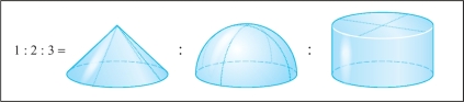
To honor this great man, Marcellus erected a tomb for Archimedes on which, according to Archimedes’ own wishes, were depicted a cone, a sphere, and a cylinder (Figure 7.33).
Archimedes was incredibly proud of his calculation of the volume and surface area of the sphere, which justifiably were seen as truly outstanding accomplishments for their time. As in his works on centers of gravity, for which he provided no clear definition, Archimedes was able to compute the surface area of the sphere without having a clear definition of precisely what it was. However, as with many mathematical works, one knows the answer long before a proof or even the correct definition can be found.
The problem of properly defining surface areas is a difficult one. To Archimedes’ credit, a careful theory of surface areas was not achieved until the twentieth century, after a long development that began in the seventeenth century with the discovery of calculus.
390
Christiaan Huygens (1629–1695) was the first person since Archimedes to give results on the areas of special surfaces beyond the sphere, and he obtained the areas of portions of surfaces of revolution, such as the paraboloid and hyperboloid.
The brilliant and prolific mathematician Leonhard Euler (1707–1783) presented the first fundamental work on the theory of surfaces in 1760 with Recherches sur la courbure des surfaces. However, it was in 1728, in a paper on shortest paths on surfaces, that Euler defined a surface as a graph \(z=f \hbox{(}x\hbox{,} y\hbox{)}\). Euler was interested in studying the curvature of surfaces, and in 1771 he introduced the notion of the parametric surfaces that are described in this section.
After the rapid development of calculus in the early eighteenth century, formulas for the lengths of curves and areas of surfaces were developed. Although we do not know when all the area formulas presented in thissection first appeared, they were certainly common by the end of the eighteenth century. The underlying concepts of the length of a curve and the area of a surface were understood intuitively before this time, and the use of formulas from calculus to compute areas was considered a great achievement.
Augustin-Louis Cauchy (1789–1857) was the first to take the step of defining the quantities of length and surface areas by integrals as we have done in this book. The question of defining surface area independent of integrals was taken up somewhat later, but this posed many difficult problems that were not properly resolved until this century.
The Spheres of Archimedes can be seen throughout nature, from the shapes of stars and planets to that of soap bubbles. Figure 7.34 shows a boy blowing a soap bubble.
Bubble blowing is an old pastime. There is even an Etruscan Vase in the Louvre on which children are portrayed blowing bubbles. Have you ever wondered why soap bubbles are round and not cubical? Analogously, why are the planets and sun round? What really determines shape and form in our universe?
391
Answers to these questions involve central concepts in our book, namely, problems of maxima and minima, and in the case of soap bubbles problems of area and volume. Soap bubbles are round because nature is economical. The spherical shape is the shape of the unique surface of least possible area containing a fixed volume (which in the case of a bubble is air).
Mathematical problems of this kind belong to a subject called The Calculus of Variations, a subject almost as old as The Calculus itself.
For more information, consult our Internet supplement or the book The Parsimonious Universe by Hildebrandt and Tromba (Springer-Verlag, 1995).