8.6 Differential Forms
476
The theory of differential forms provides an elegant way of formulating Green’s, Stokes’, and Gauss’ theorems as one statement, the fundamental theorem of calculus. The birth of the concept of a differential form is another dramatic example of how mathematics speaks to mathematicians and drives its own development. These three theorems are, in reality, generalizations of the fundamental theorem of calculus of Newton and Leibniz for functions of one variable, \[ \int^b_a f^{\prime} (x)\, {\it {\,d} x}= f(b) - f(a) \] to two and three dimensions.
Recall that Bernhard Riemann created the concept of \(n\)-dimensional spaces. If the fundamental theorem of calculus was truly fundamental, then it should generalize to arbitrary dimensions. But wait! The cross product, and therefore the curl, does not generalize to higher dimensions, as we remarked in footnote 3, in Section 1.3. Thus, some new idea is needed.
Recall that Hamilton searched for almost 15 years for his quaternions, which ultimately led to the discovery of the cross product. What is the nonexistence of a cross product in higher dimensions telling us? If the fundamental theorem of calculus is the core concept, this suggests the existence of a mathematical language in which it can be formulated in \(n\)-dimensions. In order to achieve this, mathematicians realized that they were forced to move away from vectors and on to the discovery of dual vectors and an entirely new mathematical object, a differential form. In this new language, all of the theorems of Green, Stokes, and Gauss have the same elegant and extraordinarily simple form.
Simply and very briefly stated, an expression of the type \(P{\it {\,d} x} + Q\,{\it dy}\) is a 1-form, or a differential one-form on a region in the xy plane, and F dx dy is a 2-form. Analogously, we can define the notion of an \(n\)-form. There is an operation \(d\), which takes \(n\)-forms to \(n + 1\)-forms. It is like a generalized curl and has the property that for \(\omega = P\, {\it dx} + Q {\it dy}\), we have \[ d \omega = \left( \frac{\partial\! Q}{\partial x} - \frac{\partial\! P}{\partial y}\right)\!\! {\it {\,d} x}\, {\it dy} \] and so in this notation, Green’s theorem becomes \[ \int_{\partial\! D} \omega = \int_D d\omega, \] which, interestingly, just switches the boundary operator \(\partial\!\) with the \(d\) operator. However, differential forms are more than just notation. They create a beautiful theory that generalizes to \(n\)-dimensions.
477
In general, if \(M\) is an oriented surface of dimension \(n\) with an (\(n - 1\))-dimensional boundary \(\partial\! M\) and if \(\omega\) is an (\(n - 1\))-form on \(M\), then the fundamental theorem of calculus (also called the generalized Stokes’ theorem) reads \[ \fbox{{\(\displaystyle\int_{\partial\! M} \omega =\int _{M} d\omega\).}} \]
A useful thing for you to contemplate at this stage is the sense in which the fundamental theorem of calculus becomes a special instance of this result.
In this section, we shall give a very elementary exposition of the theory of forms. Because our primary goal is to show that the theorems of Green, Stokes, and Gauss can be unified under a single theorem, we shall be satisfied with less than the strongest possible version of these theorems. Moreover, we shall introduce forms in a purely axiomatic and nonconstructive manner, thereby avoiding the tremendous number of formal algebraic preliminaries that are usually required for their construction. To the purist our approach will be far from complete, but to the student it may be comprehensible. We hope that this will motivate some students to delve further into the theory of differential forms.
We shall begin by introducing the notion of a 0-form.
0-Forms
Let \(K\) be an open set in \({\mathbb R}^3\). A 0-form on \(K\) is a real-valued function \(f{:}\,K\to {\mathbb R}\). When we differentiate \(f\) once, it is assumed to be of class \(C^1\), and \(C^2\) when we differentiate twice.
Given two 0-forms \(f_1\) and \(f_2\) on \(K\), we can add them in the usual way to get a new 0-form \(f_1+f_2\) or multiply them to get a 0-form \(f_1f_2\).
example 1
\(f_1(x,y,z)=xy+yz\) and \(f_2(x,y,z)=y\sin xz\) are 0-forms on \({\mathbb R}^3\): \[ (f_1+f_2)(x,y,z)=xy+yz+y\sin xz \] and \[ (f_1f_2)(x,y,z)=y^2 x\sin xz+y^2z\sin xz. \]
1-Forms
478
The basic 1-forms are the expressions \({\it dx},{\it dy}\), and \(dz\). At present we consider these to be only formal symbols. A 1-form \(\omega\) on an open set \(K\) is a formal linear combination \[ \omega=P(x,y,z)\,{\it {\,d} x}+Q(x,y,z)\,{\it dy}+R(x,y,z){\,d} z, \] or simply \[ \omega=P{\it {\,d} x}+Q\,{\it dy}+R{\,d} z, \] where \(P,Q\), and \(R\) are real-valued functions on \(K\). By the expression \(P{\it {\,d} x}\) we mean the 1-form \(P{\it {\,d} x}+0\,{\cdot}\,{\it dy}+0\,{\cdot}\, {\,d} z\), and similarly for \(Q\,{\it dy}\) and \(R{\,d} z\). Also, the order of \(P{\it {\,d} x}, Q\,{\it dy}\), and \(R{\,d} z\) is immaterial, and so \[ P{\it {\,d} x}+Q\,{\it dy}+R{\,d} z=R{\,d} z+P{\it {\,d} x}+Q\,{\it dy}, \hbox{etc.} \]
Given two 1-forms \(\omega_1=P_1{\it {\,d} x}+Q_1{\it dy}+R_1{\,d} z\) and \(\omega_2=P_2{\it {\,d} x}+Q_2{\it dy}+R_2{\,d} z\), we can add them to get a new 1-form \(\omega_1+\omega_2\) defined by \[ \omega_1+\omega_2=(P_1+P_2)\,{\it {\,d} x}+(Q_1+Q_2)\,{\it dy}+(R_1+R_2){\,d} z, \] and given a 0-form \(f\), we can form the 1-form \(f\omega_1\) defined by \[ f\omega_1=(f\! P_1)\,{\it {\,d} x}+(f\! Q_1)\,{\it dy}+(f\! R_1){\,d} z. \]
example 2
Let \(\omega_1=(x+y^2)\,{\it {\,d} x}+(zy)\,{\it dy}+(e^{xyz}){\,d} z\) and \(\omega_{2}=\sin y{\it {\,d} x}+\sin x{\it dy}\) be 1-forms. Then \[ \omega_1+\omega_2=(x+y^2+\sin y)\,{\it {\,d} x}+(zy+\sin x)\,{\it dy} +(e^{xyz}){\,d} z. \]
If \(f(x,y,z)=x\), then \[ f\omega_2=x\sin y{\it {\,d} x}+x\sin x{\it dy}. \]
2-Forms
The basic 2-forms are the formal expressions \({\it {\,d} x}\, {\it dy}, {\it dy} {\,d} z\), and \({\,d} z{\it {\,d} x}\). These expressions should be thought of as products of \({\it {\,d} x}\) and \({\it dy},{\it dy}\) and \({\,d} z\), and \({\,d} z\) and \({\it {\,d} x}\).
A 2-form \(\eta\) on \(K\) is a formal expression \[ \eta=F{\it {\,d} x}\,{\it dy}+G\,{\it dy}{\,d} z+H{\,d} z{\it {\,d} x}, \] where \(F,G\), and \(H\) are real-valued functions on \(K\). The order of \(F{\it {\,d} x}\,{\it dy}, G\,{\it dy}{\,d} z\), and \(H{\,d} z{\it {\,d} x}\) is immaterial; for example, \[ F{\it {\,d} x}\,{\it dy}+G\,{\it dy}\,{\,d} z+H{\,d} z{\it {\,d} x}=H{\,d} z\,{\it {\,d} x}+F{\it {\,d} x}\,{\it dy}+G\,{\it dy}\,{\,d} z,\hbox{etc.} \]
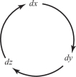
At this point it is useful to note that in a 2-form the basic 1-forms \({\it {\,d} x},{\it dy}\), and \(dz\) always appear in cyclic pairs (see Figure 8.40), that is, \({\it {\,d} x}\,{\it dy},{\it dy}\,{\,d} z\), and \({\,d} z{\it {\,d} x}\).
479
By analogy with 0-forms and 1-forms, we can add two 2-forms \[ \eta_i=F_i{\it {\,d} x}\,{\it dy}+G_i\,{\it dy}\,{\,d} z+H_i{\,d} z{\it {\,d} x}, \] \(i =1\) and 2, to obtain a new 2-form, \[ \eta_1+\eta_2=(F_1+F_2)\,{\it {\,d} x}\,{\it dy}+ (G_1 +G_2)\, {\it dy}\, {\,d} z + (H_1 + H_2) {\,d} z {\it {\,d} x}. \]
Similarly, if \(f\) is a 0-form and \(\eta\) is a 2-form, we can take the product \[ f\! \eta=(f\! F)\,{\it {\,d} x}\,{\it dy}+(f\! G)\,{\it dy}\,{\,d} z+(f\! H){\,d} z{\it {\,d} x}. \]
Finally, by the expression \(F{\it {\,d} x}\,{\it dy}\) we mean the 2-form \(F{\it {\,d} x}\,{\it dy}+0\,{\cdot}\, {\it dy}\,{\,d} z+0\,{\cdot}\, {\,d} z{\it {\,d} x}\).
example 3
The expressions \[ \eta_1=x^2{\it {\,d} x}\,{\it dy}+ y^3x\,{\it dy}\,{\,d} z+\sin zy{\,d} z{\it {\,d} x} \] and \[ \eta_2=y\,{\it dy}\,{\,d} z \] are 2-forms. Their sum is \[ \eta_1+\eta_2=x^2{\it {\,d} x}\,{\it dy}+(y^3x+y)\,{\it dy}\, {\,d} z+\sin zy {\,d} z{\it {\,d} x}. \]
If \(f(x,y,z)=xy\), then \[ \quad f\eta_2=xy^2{\it dy}\,{\,d} z. \]
3-Forms
A basic 3-form is a formal expression \({\it {\,d} x}\,{\it dy}\,{\,d} z\) (in this specific cyclic order, as in Figure 8.40). A 3-form \(\nu\) on an open set \(K\subset {\mathbb R}^3\) is an expression of the form \(\nu=f(x,y,z)\,{\it {\,d} x}\,{\it dy}\,{\,d} z\), where \(f\) is a real-valued function on \(K\).
We can add two 3-forms and we can multiply them by 0-forms in the obvious way. There seems to be little difference between a 0-form and a 3-form, because both involve a single real-valued function. But we distinguish them for a purpose that will become clear when we multiply and differentiate forms.
example 4
Let \(\nu_1= y{\it {\,d} x}\,{\it dy}\,{\,d} z\), \(\nu_2=e^{x^2}{\it {\,d} x}\,{\it dy}\,{\,d} z\), and \(f(x,y,z)=xyz\). Then \(\nu_1+\nu_2= (y+e^{x^2})\,{\it {\,d} x}\,{\it dy}\,{\,d} z\) and \(f\nu_1=y^2xz{\it {\,d} x}\,{\it dy}\,{\,d} z\).
Although we can add two 0-forms, two 1-forms, two 2-forms, or two 3-forms, we do not need to add a \(k\)-form and a \(j\)-form if \(k\neq j\). For example, we shall not need to write \[ f(x,y,z)\,{\it {\,d} x}\,{\it dy}+g\,(x,y,z){\,d} z. \]
Now that we have defined these formal objects (forms), we can legitimately ask what they are good for, how they are used, and, perhaps most important, what they mean. The answer to the first question will become clear as we proceed, but we can immediately describe how to use and interpret them.
A real-valued function on a domain \(K\) in \({\mathbb R}^3\) is a rule that assigns a real number to each point in \(K\). Differential forms are, in some sense, generalizations of the real-valued functions we have studied in calculus. In fact, 0-forms on an open set \(K\) are just functions on \(K\). Thus, a 0-form \(f\) takes points in \(K\) to real numbers.
480
We should like to interpret differential \(k\)-forms (for \(k\geq 1\)) not as functions on points in \(K\), but as functions on geometric objects such as curves and surfaces. Many of the early Greek geometers viewed lines and curves as being made up of infinitely many points, and planes and surfaces as being made up of infinitely many curves. Consequently, there is at least some historical justification for applying this geometric hierarchy to the interpretation of differential forms.
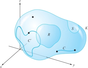
Given an open subset \(K\subset {\mathbb R}^3\), we shall distinguish four types of subsets of \(K\) (see Figure 8.41):
- (i) points in \(K\),
- (ii) oriented simple curves and oriented simple closed curves, \(C\), in \(K\),
- (iii) oriented surfaces, \(S\subset K\),
- (iv) elementary subregions, \(R\subset K\).
The Integral of 1-Forms Over Curves
We shall begin with 1-forms. Let \[ \omega=P(x,y,z)\,{\it {\,d} x}+Q(x,y,z)\,{\it dy}+R(x,y,z){\,d} z \] be a 1-form on \(K\) and let \(C\) be an oriented simple curve as in Figure 8.42. The real number that \(\omega\) assigns to \(C\) is given by the formula \begin{equation*} \int_C\omega=\int_CP(x,y,z)\,{\it {\,d} x}+Q(x,y,z)\,{\it dy}+R(x,y,z){\,d} z.\tag{1} \end{equation*}
Recall (see Section 7.2) that this integral is evaluated as follows. Suppose that \({\bf c}{:}\,[a,b]\to K, {\bf c}(t)=(x(t),y(t),z(t))\) is an orientation-preserving parametrization of \(C\). Then \begin{eqnarray*} \int_C\omega=\int_{\bf c}\omega &=& \int_a^b\bigg[P(x(t),y(t),z(t)) \,{\cdot}\,\frac{{\it dx}}{{\it dt}}\\[4pt] &&\quad + Q(x(t),y(t),z(t))\,{\cdot}\,\frac{{\it dy}}{{\it dt}} + R(x(t),y(t),z(t))\,{\cdot}\,\frac{dz}{{\it dt}}\bigg]\,{\it dt}. \end{eqnarray*}
Theorem 1 of Section 7.2 guarantees that \(\int_C\omega\) does not depend on the choice of the parametrization \({\bf c}\).
We can thus interpret a 1-form \(\omega\) on \(K\) as a rule assigning a real number to each oriented curve \(C\subset K\); a 2-form \(\eta\) will similarly be seen to be a rule assigning a real number to each oriented surface \(S\subset K\); and a 3-form \(\nu\) will be a rule assigning a real number to each elementary subregion of \(K\). The rules for associating real numbers with curves, surfaces, and regions are completely contained in the formal expressions we have defined.
481
example 5
Let \(\omega=xy{\it {\,d} x}+y^2{\it dy}+{\,d} z\) be a 1-form on \({\mathbb R}^3\) and let \(C\) be the oriented simple curve in \({\mathbb R}^3\) described by the parametrization \({\bf c}(t)=(t^2,t^3,1),0\leq t\leq 1\). \(C\) is oriented by choosing the positive direction of \(C\) to be the direction in which \({\bf c}(t)\) traverses \(C\) as \(t\) goes from 0 to 1. Then, by formula (1), \[ \int_C\omega = \int_0^1 [t^5(2t) + t^6(3t^2) + 0]\,{\it {\,d} t} = \int_0^1 (2t^6+3t^8)\,{\it dt}=\frac{13}{21}. \]
Thus, this 1-form \(\omega\) assigns to each oriented simple curve and each oriented simple closed curve \(C\) in \({\mathbb R}^3\) the number \(\int_C\omega\).
The Integral of 2-Forms Over Surfaces
A 2-form \(\eta\) on an open set \(K\subset {\mathbb R}^3\) can similarly be interpreted as a function that associates a real number with each oriented surface \(S\subset K\). This is accomplished by means of the notion of integration of 2-forms over surfaces. Let \[ \eta=F(x,y,z)\,{\it {\,d} x}\,{\it dy}+G(x,y,z)\,{\it dy}\,{\,d} z+H(x,y,z){\,d} z{\it {\,d} x} \] be a 2-form on \(K\), and let \(S\subset K\) be an oriented surface parametrized by a function \({\Phi}{:}\,D\to {\mathbb R}^3\), \(D\subset {\mathbb R}^2,{\Phi}(u,v)=(x(u,v),y(u,v),z(u,v))\) (see Section 7.3).
Definition
If \(S\) is such a surface and \(\eta\) is a 2-form on \(K\), we define \({\intop\!\!\!\intop}_S\eta\) by the formula \begin{equation*} \begin{array}{rcl} \displaystyle\intop\!\!\!\intop\nolimits_{S}\eta & = & \displaystyle\intop\!\!\!\intop\nolimits_{S} F{\it {\,d} x}\,{\it dy}+G\,{\it dy}\,{\,d} z+H{\,d} z\,{\it {\,d} x}\\[11pt] & = & \displaystyle\intop\!\!\!\intop\nolimits_{D}\bigg[F(x(u,v),y(u,v),z(u,v))\,{\cdot}\, \displaystyle\frac{\partial (x,y)}{\partial (u,v)}\\[11pt] && + \ G(x(u,v),y(u,v),z(u,v))\,{\cdot}\, \displaystyle\frac{\partial (y,z)}{\partial (u,v)}\\[11pt] & & +\ H(x(u,v),y(u,v),z(u,v))\,{\cdot}\, \displaystyle\frac{\partial (z,x)}{\partial (u,v)}\bigg]du{\,d} v, \end{array}\tag{2} \end{equation*} where \[ \frac{\partial (x,y)}{\partial (u,v)}=\left| \begin{array}{l@{\quad}r} \displaystyle \frac{\partial x}{\partial u} & \displaystyle \frac{\partial x}{\partial v}\\[9pt] \displaystyle \frac{\partial y}{\partial u} & \displaystyle \frac{\partial y}{\partial v} \end{array}\right|,\qquad \frac{\partial (y,z)}{\partial (u,v)}=\left| \begin{array}{l@{\quad}r} \displaystyle \frac{\partial y}{\partial u} & \displaystyle \frac{\partial y}{\partial v}\\[9pt] \displaystyle \frac{\partial z}{\partial u} & \displaystyle \frac{\partial z}{\partial v} \end{array}\right|,\qquad \frac{\partial (z,x)}{\partial (u,v)}=\left| \begin{array}{l@{\quad}r} \displaystyle \frac{\partial z}{\partial u} & \displaystyle \frac{\partial z}{\partial v}\\[9pt] \displaystyle \frac{\partial x}{\partial u} & \displaystyle \frac{\partial x}{\partial v} \end{array}\right|. \]
If \(S\) is composed of several pieces \(S_i,i=1,\ldots,k\), as in Figure 8.33, each with its own parametrization \({\Phi}_i\), we define \[ \intop\!\!\!\intop\nolimits_{S}\eta=\sum_{i=1}^k\intop\!\!\!\intop\nolimits_{{S_i}}\eta. \]
We must verify that \({\intop\!\!\!\intop}_S\eta\) does not depend on the choice of parametrization \({\Phi}\). This result is essentially (but not obviously) contained in Theorem 4, Section 7.6.
482
example 6
Let \(\eta=z^2{\it {\,d} x}\,{\it dy}\) be a 2-form on \({\mathbb R}^3\), and let \(S\) be the upper unit hemisphere in \({\mathbb R}^3\). Find \({\intop\!\!\!\intop}_S\eta\).
solution Let us parametrize \(S\) by \[ {\Phi}(u,v)=(\sin u\cos v,\sin u\sin v,\cos u), \] where \((u,v)\in D=[0,\pi/2]\times [0,2\pi]\). By formula (2), \[ \intop\!\!\!\intop\nolimits_{S}\eta=\intop\!\!\!\intop\nolimits_{D}\cos^2u\left[\frac{\partial (x,y)}{\partial (u,v)}\right] du{\,d} v, \] where \begin{eqnarray*} \frac{\partial (x,y)}{\partial (u,v)} &=& \bigg|\, \begin{array}{l@{\quad}r} \cos u\cos v & -\!\sin u\sin v\\[6pt] \cos u\sin v & \sin u\cos v \end{array}\,\bigg|\\[5pt] & = & \sin u\cos u\cos^2 v+\cos u\sin u\sin^2 v=\sin u\cos u. \end{eqnarray*}
Therefore, \begin{eqnarray*} \intop\!\!\!\intop\nolimits_{S}\eta &=& \intop\!\!\!\intop\nolimits_{D} \cos^2 u\cos u\sin u{\,d} u{\,d} v\\[6pt] &=& \int_0^{2\pi}\int_0^{\pi/2}\cos^3 u\sin u{\,d} u{\,d} v=\int_0^{2\pi} \left[-\frac{\cos^4 u}{4}\right]_0^{\pi/2}dv=\frac{\pi}{2}. \\[-27pt] \end{eqnarray*}
example 7
Evaluate \({\intop\!\!\!\intop}_S x\,{\it dy}\,{\,d} z+y{\it {\,d} x}\,{\it dy}\), where \(S\) is the oriented surface described by the parametrization \(x=u+v,y=u^2-v^2,z=uv\), where \((u,v)\in D=[0,1]\times [0,1]\).
solution By definition, we have \begin{eqnarray*} \frac{\partial (y,z)}{\partial (u,v)} &=& \bigg|\,\begin{array}{c@{\quad}c} 2u & -2v\\[4pt] v & u \end{array}\,\bigg|=2\,(u^2+v^2);\\[6pt] \frac{\partial (x,y)}{\partial (u,v)} &=& \bigg|\,\begin{array}{c@{\quad}c} 1 & 1\\[4pt] 2u & -2v\end{array}\,\bigg|=-2\,(u+v). \end{eqnarray*}
Consequently, \begin{eqnarray*} \intop\!\!\!\intop\nolimits_{S}x\,{\it dy}\,{\,d} z +y{\it {\,d} x}\,{\it dy} &=& \intop\!\!\!\intop\nolimits_{D}[(u+v)(2)(u^2+v^2)+(u^2-v^2)(-2)(u+v)]{\,d} u{\,d} v\\[7pt] &=& 4\intop\!\!\!\intop\nolimits_{D}(v^3+uv^2){\,d} u{\,d} v=4\int_0^1\int_0^1(v^3+uv^2){\,d} u{\,d} v\\[7pt] &=& 4\int_0^1\left[uv^3+\frac{u^2v^2}{2}\right]_0^1dv=4\int_0^1 \left(v^3+\frac{v^2}{2}\right)\!\!{\,d} v\\[7pt] &=& \left[v^4+\frac{2v^3}{3}\right]_0^1=1+\frac{2}{3}=\frac{5}{3}. \\[-27pt] \end{eqnarray*}
The Integral of 3-Forms Over Regions
483
Finally, we must interpret 3-forms as functions on the elementary subregions of \(K\). Let \(v =f(x,y,z)\,{\it {\,d} x}\,{\it dy}\,{\,d} z\) be a 3-form and let \(R\subset K\) be an elementary subregion of \(K\). Then to each such \(R\subset K\) we assign the number \begin{equation*} \intop\!\!\!\intop\!\!\!\intop\nolimits_{R} v =\intop\!\!\!\intop\!\!\!\intop\nolimits_{R}f(x,y,z)\,{\it {\,d} x}\,{\it dy}\,{\,d} z,\tag{3} \end{equation*} which is just the ordinary triple integral of \(f\) over \(R\), as described in Section 5.5.
example 8
Suppose \(v=(x+z)\,{\it {\,d} x}\,{\it dy}\,{\,d} z\) and \(R=[0,1]\times [0,1]\times [0,1]\). Evaluate \({\intop\!\!\!\intop\!\!\!\intop}_R v\).
solution We compute: \begin{eqnarray*} \intop\!\!\!\intop\!\!\!\intop\nolimits_{R} v &=& \intop\!\!\!\intop\!\!\!\intop\nolimits_{R}(x+z)\,{\it {\,d} x}\,{\it dy}\,{\,d} z=\int_0^1\int_0^1\int_0^1(x+z)\, {\it {\,d} x}\,{\it dy}\,{\,d} z\\[5pt] &=& \int_0^1\int_0^1\left[\frac{x^2}{2}+zx\right]_0^1{\it dy}\,{\,d} z= \int_0^1\int_0^1\left(\frac{1}{2}+z\right)\,{\it dy}\,{\,d} z=\int_0^1\left(\frac{1}{2}+z\right)dz\\[5pt] &=& \left[\frac{z}{2}+\frac{z^2}{2}\right]_0^1=1. \\[-28pt] \end{eqnarray*}
The Algebra of Forms
We now discuss the algebra (or rules of multiplication) of forms that, together with differentiation of forms, will enable us to state Green’s, Stokes’, and Gauss’ theorems in terms of differential forms.
If \(\omega\) is a \(k\)-form and \(\eta\) is an \(l\)-form on \(K,0\leq k+l\leq 3\), there is a product called the wedge product \(\omega \wedge \eta\) of \(\omega\) and \(\eta\) that is a \(k+l\) form on \(K\). The wedge product satisfies the following laws:
- (i) For each \(k\) there is a zero \(k\)-form 0 with the property that \(0+\omega=\omega\) for all \(k\)-forms \(\omega\) and \(0\wedge\eta=0\) for all \(l\)-forms \(\eta\) if \(0\leq k+l\leq 3\).
- (ii) (Distributivity) If \(f\) is a 0-form, then \[ (f\omega_1+\omega_2)\wedge \eta=f(\omega_1\wedge\eta)+(\omega_2\wedge\eta). \]
- (iii) (Anticommutativity) \(\omega\wedge\eta=(-1)^{kl}(\eta\wedge\omega)\).
- (iv) (Associativity) If \(\omega_1,\omega_2,\omega_3\) are \(k_1,k_2,k_3\) forms, respectively, with \(k_1 + k_2 + k_3\leq 3\), then \[ \omega_1\wedge(\omega_2\wedge\omega_3)=(\omega_1\wedge\omega_2)\wedge\omega_3. \]
- (v) (Homogeneity with respect to functions) If \(f\) is a 0-form, then \[ \omega\wedge(f\eta)=(f\omega)\wedge\eta=f(\omega\wedge\eta). \] Notice that rules (ii) and (iii) actually imply rule (v).
- (vi) The following multiplication rules for 1-forms hold: \begin{eqnarray*} &&\displaystyle {\it {\,d} x}\wedge {\it dy} = {\it {\,d} x}\,{\it dy}\\[2pt] &&\displaystyle {\it dy}\wedge {\it {\,d} x} =-{\it {\,d} x}\,{\it dy} =(-1)({\it {\,d} x}\wedge {\it dy})\\[2pt] &&\displaystyle {\it dy}\wedge {\,d} z = {\it dy}\,{\,d} z =(-1)({\,d} z\wedge {\it dy})\\[2pt] &&\displaystyle {\,d} z\wedge {\it {\,d} x} = {\,d} z\,{\it {\,d} x} =(-1)({\it {\,d} x}\wedge {\,d} z)\\[2pt] &&\displaystyle{\it {\,d} x}\wedge {\it {\,d} x}=0,\ {\it dy}\wedge{\it dy}=0,\ {\,d} z\,\wedge {\,d} z =0\\[2pt] &&\displaystyle {\it {\,d} x}\wedge ({\it dy}\wedge {\,d} z) = ({\it {\,d} x}\wedge {\it dy})\wedge{\,d} z= {\it {\,d} x}\,{\it dy}{\,d} z. \end{eqnarray*}
- (vii) If \(f\) is a 0-form and \(\omega\) is any \(k\)-form, then \(f\wedge\omega=f\omega\).
484
Using laws (i) to (vii), we can now find a unique product of any \(l\)-form \(\eta\) and any \(k\)-form \(\omega\), if \(0\leq k+l \leq 3\).
example 9
Show that \({\it {\,d} x}\wedge{\it dy}\,{\,d} z={\it {\,d} x}\,{\it dy}\,{\,d} z\).
solution By rule (vi), \({\it dy}\,{\,d} z={\it dy}\wedge{\,d} z\). Therefore, \[ {\it {\,d} x}\wedge {\it dy}\,{\,d} z={\it {\,d} x}\wedge({\it dy}\wedge {\,d} z) ={\it {\,d} x}\,{\it dy}\,{\,d} z. \]
example 10
If \(\omega=x{\it {\,d} x}+y\,{\it dy}\) and \(\eta=zy{\it {\,d} x}+xz\,{\it dy}+xy{\,d} z\), find \(\omega\wedge \eta\).
solution Computing \(\omega\wedge\eta\), to get \begin{eqnarray*} \omega\wedge\eta &=& (x{\it {\,d} x}+y\,{\it dy})\wedge(zy\,{\it {\,d} x}+xz\,{\it dy}+xy{\,d} z)\\[2pt] &=& [(x{\it {\,d} x}+y\,{\it dy})\wedge(zy{\it {\,d} x})]+[(x{\it {\,d} x}+y\,{\it dy})\wedge(xz\,{\it dy})]\\[2pt] & & +\, [(x{\it {\,d} x}+y\,{\it dy})\wedge(xy{\,d} z)]\\[2pt] &=& xyz(d x\wedge{\it {\,d} x})+zy^2(d y\wedge{\it {\,d} x})+ x^2z(d x\wedge{\it dy})+xyz(d y\wedge{\it dy})\\[2pt] & & +\, x^2y(d x\wedge{\,d} z)+xy^2(d y\wedge{\,d} z)\\[2pt] &=& -zy^2{\it {\,d} x}\,{\it dy}+x^2z{\it {\,d} x}\,{\it dy}-x^2y{\,d} z{\it {\,d} x}+xy^2{\it dy}\,{\,d} z\\[2pt] &=& (x^2z-y^2z)\,{\it {\,d} x}\,{\it dy}-x^2y{\,d} z{\it {\,d} x}+xy^2{\it dy}\,{\,d} z. \\[-30pt] \end{eqnarray*}
example 11
If \(\omega=x{\it {\,d} x}-y\,{\it dy}\) and \(\eta=x\,{\it dy}\,{\,d} z +z{\it {\,d} x}\,{\it dy}\), find \(\omega\wedge\eta\).
solution \begin{eqnarray*} \omega\wedge\eta &=& (x{\it {\,d} x}-y\,{\it dy})\wedge(x\,{\it dy}\,{\,d} z+z{\it {\,d} x}\,{\it dy})\\[2pt] &=& [(x{\it {\,d} x}-y\,{\it dy})\wedge(x\,{\it dy}\,{\,d} z)]+[(x{\it {\,d} x}-y\,{\it dy})\wedge(z{\it {\,d} x}\,{\it dy})]\\[2pt] &=& (x^2{\it {\,d} x}\wedge{\it dy}\,{\,d} z)-(xy\,{\it dy}\wedge {\it dy}\,{\,d} z)+ (xz{\it {\,d} x}\wedge {\it {\,d} x}\,{\it dy})\\[2pt] &&-\ (yz\,{\it dy}\wedge {\it {\,d} x}\,{\it dy})\\[2pt] &=& [x^2 {\it {\,d} x}\wedge(d y\wedge{\,d} z)]-[xy\, {\it dy}\wedge(d y\wedge{\,d} z)] +\, [xz{\it {\,d} x}\wedge({\it dx}\wedge {\it dy})]\\[2pt] &&-\ [yz\, {\it dy} \wedge ({\it dx}\wedge {\it dy})]\\[2pt] &=& x^2{\it {\,d} x}\,{\it dy}{\,d} z -[xy({\it dy}\wedge {\it dy})\wedge{\,d} z] +\, [xz (d x\wedge {\it {\,d} x})\wedge{\it dy}]\\[2pt] & &-\ [yz(d y\wedge {\it {\,d} x})\wedge{\it dy}]\\[2pt] &=& x^2 {\it {\,d} x}\,{\it dy}\,{\,d} z- xy(0\wedge{\,d} z) +xz(0\wedge{\it dy})+[yz(d y\wedge {\it dy})\wedge{\it {\,d} x}]\\[2pt] &=& x^2{\it {\,d} x}\, {\it dy}\,{\,d} z. \\[-28pt] \end{eqnarray*}
The last major step in the development of this theory is to show how to differentiate forms. The derivative of a \(k\)-form is a \((k+1)\)-form if \(k<3\), and the derivative of a 3-form is always zero. If \(\omega\) is a \(k\)-form, we shall denote the derivative of \(\omega\) by \(d\omega\). The operation \(d\) has the following properties:
485
(1) If \(f{:}\,K\to {\mathbb R}\) is a 0-form, then \[ {\,d} f=\frac{\partial\! f}{\partial x}{\it {\,d} x}+\frac{\partial\! f}{\partial y}{\it dy}+\frac{\partial\! f}{\partial z}{\,d} z. \]
(2)(Linearity) If \(\omega_1\) and \(\omega_2\) are \(k\)-forms, then \[ d(\omega_1+\omega_2)={\,d} \omega_1+{\,d} \omega_2. \]
(3) If \(\omega\) is a \(k\)-form and \(\eta\) is an \(l\)-form, \[ d(\omega\wedge\eta)=(d\omega\wedge\eta)+(-1)^k(\omega\wedge d\eta). \]
(4) \(d(d\omega)=0\) and \(d({\it dx})=d({\it dy})=d(dz)=0\) or, simply, \(d^2=0\).
Properties (1) to (4) provide enough information to allow us to uniquely differentiate any form.
example 12
Let \(\omega=P(x,y,z)\,{\it {\,d} x}+Q(x,y,z)\,{\it dy}\) be a 1-form on some open set \(K\subset {\mathbb R}^3\). Find \(d\omega\).
solution \[ \begin{array}{ll} d[P(x,y,z)\,{\it {\,d} x}+Q(x,y,z)\,{\it dy}]\\ \quad = d[P(x,y,z)\wedge {\it {\,d} x}]+ d[Q(x,y,z)\wedge {\it dy}]&\hbox{(using 2)}\\ \quad = (dP\wedge {\it {\,d} x})+[P\wedge {\,d}(d x)]+ (d Q\wedge{\it dy})+[Q\wedge {\,d}(d y)]&\hbox{(using 3)}\\[-1pt] \quad = (dP\wedge {\it {\,d} x})+(dQ\wedge{\it dy})&\hbox{(using 4)}\\[6pt] \quad =\left(\frac{\partial\! P}{\partial x}{\it {\,d} x}+ \frac{\partial\! P}{\partial y}{\it dy}+ \frac{\partial\! P}{\partial z}{\,d} z\right)\wedge{\it {\,d} x}&\\[6pt] \qquad +\left(\frac{\partial\! Q}{\partial x}{\it {\,d} x}+\frac{\partial\! Q}{\partial y}{\it dy}+\frac{\partial\! Q}{\partial z}{\,d} z\right)\wedge{\it dy}&\hbox{(using 1)}\\[6pt] \quad = \left(\frac{\partial\! P}{\partial x}{\it {\,d} x}\wedge{\it {\,d} x}\right)+\left(\frac{\partial\! P}{\partial y}{\it dy}\wedge{\it {\,d} x}\right)+\left(\frac{\partial\! P}{\partial z}{\,d} z\wedge{\it {\,d} x}\right)&\\[6pt] \qquad + \left(\frac{\partial\! Q}{\partial x}{\it {\,d} x}\wedge{\it dy}\right)+\left(\frac{\partial\! Q}{\partial y}{\it dy}\wedge{\it dy}\right)+\left(\frac{\partial\! Q}{\partial z}{\,d} z\wedge{\it dy}\right)&\\[6pt] \quad = -\frac{\partial\! P}{\partial y}{\it {\,d} x}\,{\it dy}+\frac{\partial\! P}{\partial z}{\,d} z{\it {\,d} x}+\frac{\partial\! Q}{\partial x}{\it {\,d} x}\,{\it dy}-\frac{\partial\! Q}{\partial z}{\it dy}{\,d} z&\\[6pt] \quad = \left(\frac{\partial\! Q}{\partial x}-\frac{\partial\! P}{\partial y}\right)\,{\it {\,d} x}\,{\it dy}+\frac{\partial\! P}{\partial z}{\,d} z{\it {\,d} x}-\frac{\partial\! Q}{\partial z}{\it dy}\,{\,d} z.& \end{array} \]
example 13
Let \(f\) be a 0-form. Using only differentiation rules (1) to (3) and the fact that \(d({\it dx})=d({\it dy})=d(dz)=0\), show that \(d(df)=0\).
solution By rule (1), \[ df=\frac{\partial\! f}{\partial x}{\it {\,d} x}+\frac{\partial\! f}{\partial y}{\it dy}+\frac{\partial\! f}{\partial z}{\,d} z, \] and so \[ d(df)=d\left(\frac{\partial\! f}{\partial x}{\it {\,d} x}\right)+d\left(\frac{\partial\! f}{\partial y}{\it dy}\right)+d\left(\frac{\partial\! f}{\partial z}{\,d} z\right). \]
486
Working only with the first term, using rule (3), we get \begin{eqnarray*} d\left(\frac{\partial\! f}{\partial x}{\it {\,d} x}\right) &=& d\left(\frac{\partial\! f}{\partial x}\wedge {\it {\,d} x}\right)=d\left(\frac{\partial\! f}{\partial x}\right)\wedge{\it {\,d} x}+\frac{\partial\! f}{\partial x}\wedge d({\it dx})\\[8pt] &=& \left(\frac{\partial^2f}{\partial x^2}{\it {\,d} x}+\frac{\partial^2f}{\partial y\,\partial x}{\it dy}+\frac{\partial^2f}{\partial z\,\partial x}{\,d} z\right)\wedge{\it {\,d} x}+0\\[8pt] &=& \frac{\partial^2f}{\partial y\,\partial x}{\it dy}\wedge{\it {\,d} x}+\frac{\partial^2 f}{\partial z\,\partial x}{\,d} z\wedge{\it {\,d} x}\\[8pt] &=& -\frac{\partial^2f}{\partial y\,\partial x}{\it {\,d} x}\,{\it dy}+\frac{\partial^2 f}{\partial z\,\partial x}{\,d} z\,{\it {\,d} x}. \end{eqnarray*}
Similarly, we find that \[ d\left(\frac{\partial\! f}{\partial y}{\it dy}\right)=\frac{\partial^2f}{\partial x\,\partial y}{\it {\,d} x}\,{\it dy}-\frac{\partial^2f}{\partial z\,\partial y}{\it dy}{\,d} z \] and \[ d\left(\frac{\partial\! f}{\partial z}{\,d} z\right)=-\frac{\partial^2f}{\partial x\,\partial z}{\,d} z{\it {\,d} x}+\frac{\partial^2f}{\partial y\,\partial z}{\it dy}{\,d} z. \]
Adding these up, we get \(d(df)=0\) by the equality of mixed partial derivatives.
example 14
Show that \(d({\it {\,d} x}\,{\it dy}),d({\it dy}\,{\,d} z)\), and \(d({\,d} z{\it {\,d} x})\) are all zero.
solution To prove the first case, we use property (3): \[ d(d x\,{\it dy})=d({\it dx}\wedge {\it dy})=[d({\it dx})\wedge {\it dy} -{\it dx}\wedge d({\it dy})]=0. \]
The other cases are similar.
example 15
If \(\eta=F(x,y,z)\,{\it {\,d} x}\,{\it dy}+G(x,y,z)\,{\it dy}\,{\,d} z+H(x,y,z){\,d} z\,{\it {\,d} x}\), find \(d\eta\).
solution By property (2), \[ d\eta=d(F{\it {\,d} x}\,{\it dy})+{\,d}(G\,{\it dy}\,{\,d} z)+d(H{\,d} z\,{\it {\,d} x}). \]
We shall compute \(d(F{\it {\,d} x}\,{\it dy})\). Using property (3) again, we get \[ d(F{\it {\,d} x}\,{\it dy})=d(F\wedge {\it {\,d} x}\,{\it dy})=dF\wedge ({\it dx}\,{\it dy})+F\wedge d({\it dx}\,{\it dy}). \]
By Example 14, \(d({\it dx}\,{\it dy})=0\), so we are left with \begin{eqnarray*} dF\wedge (d x\,{\it dy})&=& \left(\frac{\partial\! F}{\partial x}{\it {\,d} x}+\frac{\partial\! F}{\partial y}{\it dy}+\frac{\partial\! F}{\partial z}{\,d} z\right)\wedge({\it dx}\wedge {\it dy})\\[8pt] &=& \left[\frac{\partial\! F}{\partial x}{\it dx}\wedge ({\it dx}\wedge {\it dy})\right]+\left[\frac{\partial\! F}{\partial y}{\it dy}\wedge ({\it dx}\wedge {\it dy})\right]\\[8pt] &&+ \left[\frac{\partial\! F}{\partial z}dz\wedge ({\it dx}\wedge {\it dy})\right].\\[-9pt] \end{eqnarray*}
487
Now \begin{eqnarray*} {\it dx}\wedge ({\it dx}\wedge {\it dy}) &=& ({\it dx}\wedge {\it dx})\wedge {\it dy}=0\wedge {\it dy}=0,\\ {\it dy}\wedge ({\it dx}\wedge {\it dy}) &=& -{\it dy}\wedge ({\it dy}\wedge {\it dx})\\ &=& -({\it dy}\wedge {\it dy})\wedge {\it dx}=0\wedge {\it dx}=0,\\[-15pt] \end{eqnarray*} and \[ dz\wedge ({\it dx}\wedge {\it dy})=(-1)^2({\it dx}\wedge {\it dy})\wedge dz={\it dx}\, {\it dy}\, {\,d} z. \]
Consequently, \[ d(F{\it {\,d} x}\,{\it dy})=\frac{\partial\! F}{\partial z}{\it {\,d} x}\,{\it dy}\,{\,d} z. \]
Analogously, we find that \[ d(G\,{\it dy}\,{\,d} z)=\frac{\partial G}{\partial x}{\it {\,d} x}\,{\it dy}\,{\,d} z\hbox{and} d(H{\,d} z{\it {\,d} x})=\frac{\partial\! H}{\partial y}{\it {\,d} x}\,{\it dy}\,{\,d} z. \]
Therefore, \[ d\eta=\left(\frac{\partial\! F}{\partial z}+\frac{\partial G}{\partial x}+\frac{\partial\! H}{\partial y}\right)\!\!{\it {\,d} x}\,{\it dy}\,{\,d} z. \]
We have now developed all the concepts needed to reformulate Green’s, Stokes’, and Gauss’ theorems in the language of forms.
Theorem 11 Green’s Theorem
Let \(D\) be an elementary region in the \(xy\) plane, with \(\partial\! D\) given the counterclockwise orientation. Suppose \(\omega=P(x,y)\,{\it {\,d} x} +Q(x,y)\,{\it dy}\) is a 1-form on some open set \(K\) in \({\mathbb R}^3\) that contains \(D\). Then \[ \int_{\partial\! D}\omega=\intop\!\!\!\intop\nolimits_{D} {\,d}\omega. \]
Here \(d\omega\) is a 2-form on \(K\) and \(D\) is in fact a surface in \({\mathbb R}^3\) parametrized by \({\Phi}{:}\,D\to {\mathbb R}^3, {\Phi}(x,y)=(x,y,0)\). Because \(P\) and \(Q\) are explicitly not functions of \(z\), then \(\partial\! P/\partial z\) and \(\partial\! Q/\partial z=0\), and by Example 12, \(d\omega=(\partial\! Q/\partial x-\partial\! P/\partial y)\,{\it {\,d} x}\,{\it dy}\). Consequently, Theorem 13 means nothing more than that \[ \int_{\partial\! D}P {\it {\,d} x}+Q\,{\it dy}=\intop\!\!\!\intop\nolimits_{D}\left( \frac{\partial\! Q}{\partial x}-\frac{\partial\! P}{\partial y}\right)\,{\it dx}\,{\it dy}, \] which is precisely Green’s theorem. Hence, Theorem 13 holds. Likewise, we have the following theorems.
Theorem 12 Stokes’ Theorem
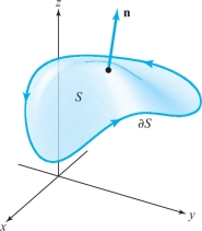
Let \(S\) be an oriented surface in \({\mathbb R}^3\) with a boundary consisting of a simple closed curve \(\partial\! S\) (Figure 8.42) oriented as the boundary of \(S\) (see Figure 8.11). Suppose that \(\omega\) is a 1-form on some open set \(K\) that contains \(S\). Then \[ \int_{\partial S}\omega=\intop\!\!\!\intop\nolimits_{S} d\omega. \]
488
Theorem 13 Gauss’ Theorem
Let \({W}\subset {\mathbb R}^3\) be an elementary region with \(\partial\! {W}\) given the outward orientation (see Section 8.5). If \(\eta\) is a 2-form on some region \(K\) containing \(W\), then \[ \intop\!\!\!\intop\nolimits_{{\partial\! W}}\eta=\intop\!\!\!\intop\!\!\!\intop\nolimits_{W} d\eta. \]
The reader has probably noticed the strong similarity in the statements of these theorems. In the vector-field formulations, we used divergence for regions in \({\mathbb R}^3\) (Gauss’ theorem) and the curl for surfaces in \({\mathbb R}^3\) (Stokes’ theorem) and regions in \({\mathbb R}^2\) (Green’s theorem). Here we just use the unified notion of the derivative of a differential form for all three theorems; and, in fact, we can state all theorems as one by introducing a little more terminology.
By an oriented 2-manifold with boundary in \({\mathbb R}^3\) we mean a surface in \({\mathbb R}^3\) whose boundary is a simple closed curve with orientation as described in Section 8.3. By an oriented 3-manifold in \({\mathbb R}^3\) we mean an elementary region in \({\mathbb R}^3\) (we assume its boundary, which is a surface, is given the outward orientation discussed in Section 8.5). We call the following unified theorem “Stokes’ theorem,” according to the current convention.
Theorem 14 General Stokes’ Theorem
Let \(M\) be an oriented \(k\)-manifold in \({\mathbb R}^3 (k = 2 \hbox{ or } 3)\) contained in some open set \(K\). Suppose \(\omega\) is \((k-1)\)-form on \(K\). Then \[ \int_{\partial\! M} \omega = \int_M {\,d} \omega. \]
Here the integral is interpreted as a single, double, or triple integral, as is appropriate. In fact, it is this form of Stokes’ theorem that generalizes to spaces of arbitrary dimension.