8.4 Conservative Fields
453
We saw in Section 7.2 that for a gradient force field \({\bf F} = {\nabla}\! f\), line integrals of \({\bf F}\) were evaluated as follows: \[ \int_{\bf c} {\bf F} \,{\cdot}\, d {\bf s} = f ( {\bf c} (b)) - f ( {\bf c} (a)). \]
The value of the integral depends only on the endpoints \({\bf c} (b)\) and \({\bf c} (a)\) of the path. In other words, if we used another path with the same endpoints, we would still get the same answer. This leads us to say that the integral is path-independent.
Gradient fields are important in many physical problems. For example, if \(V= -f\) represents a potential energy (gravitational, electrical, and so on), then \({\bf F}\) represents a force.footnote # Consider the example of a particle of mass \(m\) in the field of the earth; in this case, we take \(f\) to be \({\it GmM} /r\) or \(V=-{\it GmM}/r\), where \(G\) is the gravitational constant, \(M\) is the mass of the earth, and \(r\) is the distance from the center of the earth. The corresponding force is \({\bf F} = {-}({\it GmM}/r^3) {\bf r}= -({\it GmM}/r^2){\bf n}\), where \({\bf n}\) is the unit radial vector. Note that \({\bf F}\) fails to be defined at the point \(r=0\).
When Are Vector Fields Gradients?
We wish to characterize those vector fields that can be written as a gradient. Our task is simplified considerably by Stokes’ theorem.
Theorem 7 Conservative Fields
Let \({\bf F}\) be a \(C^1\) vector field defined on \({\mathbb R}^3\), except possibly for a finite number of points. The following conditions on \({\bf F}\) are all equivalent:
- (i) For any oriented simple closed curve \(C, \int_C {\bf F} \,{\cdot}\, d {\bf s} =0\).
- (ii) For any two oriented simple curves \(C_1\) and \(C_2\) that have the same endpoints, \[ \int_{C_1} {\bf F} \,{\cdot}\, d {\bf s} = \int_{C_2} {\bf F} \,{\cdot}\, d {\bf s}. \]
- (iii) \({\bf F}\) is the gradient of some function \(f\); that is, \({\bf F} = {\nabla}f\) (and if \({\bf F}\) has one or more exceptional points where it fails to be defined, \(f\) is also undefined there).
- (iv) \({\nabla} \times {\bf F} ={\bf 0}\).
A vector field satisfying one (and, hence, all) of the conditions (i)–(iv) is called a} conservative vector field.footnote #
454
proof
We shall establish the following chain of implications, which will prove the theorem: \[ {\rm (i)} \Rightarrow {\rm (ii)} \Rightarrow {\rm (iii)} \Rightarrow {\rm (iv)}\Rightarrow {\rm (i)}. \]
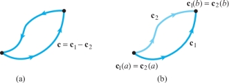
First we show that condition (i) implies condition (ii). Suppose \({\bf c}_1\) and \({\bf c}_2\) are parametrizations representing \(C_1\) and \(C_2\), with the same endpoints. Construct the closed curve \({\bf c}\) obtained by first traversing \({\bf c}_1\) and then \(-{\bf c}_2\) (Figure 8.26), or, symbolically, the curve \({\bf c} = {\bf c}_1 - {\bf c}_2\). Assuming \({\bf c}\) is simple, condition (i) gives \[ \int_{\bf c} {\bf F} \,{\cdot}\, d {\bf s} = \int_{{\bf c}_1} {\bf F} \,{\cdot}\, d {\bf s} - \int_{{\bf c}_2} {\bf F}\,{\cdot}\, d{\bf s} =0, \] and so condition (ii) holds. (If \({\bf c}\) is not simple, an additional argument, omitted here, is needed.)
Next, we prove that condition (ii) implies condition (iii). Let \(C\) be any oriented simple curve joining a point such as \((0, 0, 0)\) to \((x,y,z)\), and suppose \(C\) is represented by the parametrization \({\bf c}\) [if \((0, 0, 0)\) is the exceptional point of \({\bf F}\), we can choose a different starting point for \({\bf c}\) without affecting the argument]. Define \(f(x,y,z)\) to be \(\int_{\bf c} {\bf F} \,{\cdot}\,d {\bf s}\). By hypothesis (ii), \(f (x,y,z)\) is independent of \(C\). We shall show that \({\bf F}=\) grad \(f\). Indeed, choose \({\bf c}\) to be the path shown in Figure 8.27, so that \[ f (x,y,z) = \int_0^x F_1 (t,0,0)\, {\it dt} + \int_0^y F_2 (x,t,0) \,{\it {\,d} t} + \int_0^z F_3 (x,y,t) \,{\it {\,d} t}, \] where \({\bf F} = (F_1, F_2, F_3)\).
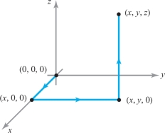
It follows from the fundamental theorem of calculus that \(\partial\! f /\partial z=F_3\). We can repeat this processing using two other paths from (0, 0, 0) to \((x,y,z)\) [for example, by drawing the lines from (0, 0, 0) to \((0,y,0)\) to \((x,y,0)\) to \((x,y,z)\)], and we can similarly show that \(\partial\! f/ \partial x = F_1\) and \(\partial\! f/ \partial y=F_2\) (see Exercise 26). Thus, \({\nabla}\! f= {\bf F}\).
Third, condition (iii) implies condition (iv), because, as proved in Section 4.4, \[ {\nabla} \times {\nabla}\! f= {\bf 0}. \]
455
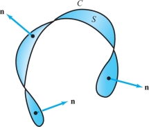
Finally, let \({\bf c}\) represent a closed curve \(C\) and let \(S\) be any surface whose boundary is \({\bf c}\) (if \({\bf F}\) has exceptional points, choose \(S\) to avoid them). Figure 8.28 indicates that we can probably always find such a surface; however, a formal proof of this would require the development of more sophisticated mathematical ideas than we can present here. By Stokes’ theorem, \[ \int_C {\bf F} \,{\cdot}\, d {\bf s} = \int_{\bf c} {\bf F} \,{\cdot}\, d {\bf s} = \intop\!\!\!\intop\nolimits_{S} ({\nabla} \times {\bf F}) \,{\cdot}\, {\bf n}\, \,{\,d} S =\intop\!\!\!\intop\nolimits_{S} (\hbox{curl }{\bf F}) \,{\cdot}\, {\bf n}\, \,{\,d} S. \]
Because \({\nabla} \times {\bf F} ={\bf 0}\), this integral vanishes, so that condition (iv) \(\Rightarrow\) condition (i).
Physical Interpretations of
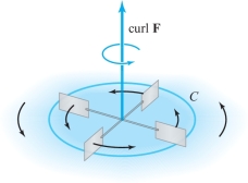
We have already seen that one interpretation of the line integral is as the work done by \({\bf F}\) in moving a particle along \(C\). A second interpretation is the notion of circulation, which we encountered at the end of the last section. Recall that in this case, we think of \({\bf F}\) as the velocity field of a fluid; that is, to each point P in space, \({\bf F}\) assigns the velocity vector of the fluid at P (in the last section, \({\bf F}\) was designated \({\bf V}\)). Take \(C\) to be a closed curve, and let \(\Delta {\bf s}\) be a small directed chord of \(C\). Then \({\bf F} \,{\cdot}\, \Delta {\bf s}\) is approximately the tangential component of \({\bf F}\) times \(\| \Delta {\bf s} \|\). The circulation \(\int_C {\bf F} \,{\cdot}\, d {\bf s}\) is the net tangential component around \(C\). A small paddle wheel placed in the fluid would rotate if it is centered at a point where \({\bf F}\) vanishes and if the circulation of the fluid is nonzero, or \(\int_C {\bf F} \,{\cdot}\, d {\bf s} \ne 0\) for small loops \(C\) (see Figure 8.29).
There is a similar interpretation in electromagnetic theory: If \({\bf F}\) represents an electric field, then a current will flow around a loop \(C\) if \(\int_C {\bf F} \,{\cdot}\, d {\bf s} \ne 0\).
By Theorem 7, a field \({\bf F}\) has no circulation if and only if \(\hbox{curl } {\bf F} = {\nabla} \times {\bf F}= {\bf 0}\). Hence, a vector field \({\bf F}\) with curl \({\bf F}= {\bf 0}\) is called irrotational. We have therefore proved that a vector field in \({\mathbb R}^3\) is irrotational if and only if it is a gradient field for some function, that is, if and only if \({\bf F} = {\nabla}\! f\). The function \(f\) is called a potential for \({\bf F}\).
456
example 1
Consider the vector field \({\bf F}\) on \({\mathbb R}^3\) defined by \[ {\bf F} (x,y,z) = y {\bf i}+ ( z \cos yz + x) {\bf j} + (y \cos yz) {\bf k}. \]
Show that \({\bf F}\) is irrotational and find a scalar potential for \({\bf F}\).
solution We compute \({\nabla} \times {\bf F}\): \begin{eqnarray*} {\nabla} \times {\bf F} &=& \left| \begin{array}{c@{\quad}c@{\quad}c} \displaystyle {\bf i} & {\bf j} & {\bf k} \\[5pt] \displaystyle \frac{\partial\!}{\partial x} & \displaystyle \frac{\partial\!}{\partial y}& \displaystyle \frac{\partial\!}{\partial z}\\[10pt] y &\quad x + z \cos yz\quad & y\ \cos yz \ \end{array} \right| \\[7pt] &=& ( \cos yz - yz \sin yz - \cos yz + yz \sin yz) {\bf i}+ (0-0) {\bf j} + (1-1) {\bf k} \\ & = & 0 {\bf i} + 0 {\bf j} + 0 {\bf k} = {\bf 0}, \end{eqnarray*} so \({\bf F}\) is irrotational. Thus, a potential exists by Theorem 7. We can find it in several ways.
Method 1. By the technique used to prove that condition (ii) implies condition (iii) in Theorem 7, we can set \begin{eqnarray*} f (x,y,z) & = & \int_0^x F_1 (t,0,0)\,{\it {\,d} t} + \int_0^y F_2 (x,t,0) \,{\it {\,d} t} + \int_0^z F_3 (x,y,t) \,{\it {\,d} t} \\[8pt] & = & \int_0^x 0\,{\it {\,d} t} + \int_0^y x \,{\it {\,d} t} + \int_0^z y \cos y t \,{\it {\,d} t} \\ [8pt] & = & 0 + xy + \sin yz = xy + \sin yz. \end{eqnarray*}
We easily verify that \({\nabla}\! f={\bf F}\), as required: \[ {\nabla}\! f = \frac{\partial\! f}{\partial x} \,{\bf i}+ \frac{\partial\! f}{\partial y}\, {\bf j}+ \frac{\partial\! f}{\partial z}\, {\bf k}= y {\bf i} + ( x +z \cos yz) {\bf j}+ (y \cos yz) {\bf k}. \]
Method 2}. Because we know that \(f\) exists, we know that we can solve the system of equations \[ \frac{\partial\! f}{\partial x} =y , \frac{\partial\! f}{\partial y} = x+ z \cos yz, \frac{\partial\! f}{\partial z} = y \cos yz, \] for \(f (x,y,z)\). These are equivalent to the simultaneous equations
- (a) \(f (x,y,z) = xy + h_1 (y,z)\)
- (b) \(f (x,y,z) = \sin yz + xy + h_2 (x,z)\)
- (c) \(f (x,y,z) =\sin yz + h_3 (x,y)\)
for functions \(h_1, h_2, h_3\) independent of \(x,y\), and \(z\) (respectively). When \(h_1(y,z)= \sin yz\), \(h_2 (x,z)=0\), and \(h_3 (x,y) = xy\), the three equations agree and so yield a potential for \({\bf F}\). However, we have only guessed at the values of \(h_1, h_2\), and \(h_3\). To derive the formula for \(f\) more systematically, we note that because \(f (x,y,z)= xy + h_1 (y,z)\) and \(\partial\! f / \partial z = y \cos yz\), we find that \[ \frac{\partial h_1 (y,z)}{\partial z} = y \cos yz \] or \[ h_1 (y,z) = \int y \cos yz {\,d} z + g (y) = \sin yz + g (y). \]
457
Therefore, substituting this back into equation (a), we get \[ f (x,y,z) = xy + \sin yz + g (y); \] but by equation (b), \[ g (y) = h_2 (x,z). \]
Because the right side of this equation is a function of \(x\) and \(z\) and the left side is a function of \(y\) alone, we conclude that they must equal some constant \(C\). Thus, \[ f (x,y,z) = xy + \sin yz + C \] and we have determined \(f\) up to a constant.
example 2
A mass \(M\) at the origin in \({\mathbb R}^3\) exerts a force on a mass \(m\) located at \({\bf r}= (x,y,z)\) with magnitude \({\it GmM}/r^2\) and directed toward the origin. Here, \(G\) is the gravitational constant, which depends on the units of measurement, and \(r = \|{\bf r} \|={\textstyle\sqrt{x^2 + y^2 + z^2}}\). If we remember that \(-{\bf r} / r\) is a unit vector toward the origin, then we can write the force field as \[ {\bf F} (x,y,z) = - \frac{{\it GmM}{\bf r}}{r^3}. \]
Show that \({\bf F}\) is irrotational and find a scalar potential for \({\bf F}\). (Notice that \({\bf F}\) is not defined at the origin, but Theorem 7 still applies, because it allows an exceptional point.)
solution First let us verify that \({\nabla} \times {\bf F} = {\bf 0}\). Referring to formula 10 in the table of vector identities in Section 4.4,we get \[ {\bf F} = - {\it GmM} \left[ {\nabla}\!\left(\frac{1}{r^3}\right) \times {\bf r} + \frac{1}{r^3} {\nabla} \times {\bf r} \right]. \]
But \({\nabla} (1/r^3) = - 3 {\bf r}/ r^5\) (see Exercise 38, Section 4.4), and so the first term vanishes, because \({\bf r} \times {\bf r} = {\bf 0}\). The second term vanishes, because \[ {\nabla} \times {\bf r} = \left| \begin{array}{c@{\quad}c@{\quad}c} {\bf i} & {\bf j} & {\bf k} \\[5pt] \displaystyle\frac{\partial\!}{\partial x} & \displaystyle\frac{\partial\!}{\partial y} & \displaystyle \frac{\partial\!}{\partial z} \\[10pt] x & y & z \end{array} \right| = \left( \frac{\partial z}{\partial y}- \frac{\partial y}{\partial z} \right) {\bf i}+ \left( \frac{\partial x}{\partial z}-\frac{\partial z}{\partial x} \right) {\bf j}+ \left( \frac{\partial y}{\partial x} -\frac{\partial x}{\partial y} \right) {\bf k} = {\bf 0}. \]
Hence, \({\nabla} \times {\bf F} = 0\) (for \({\bf r} \ne 0\)).
If we recall the formula \({\nabla} (r^n) = n r^{n-2} {\bf r}\) (again, see Exercise 38, Section 4.4), then we can read off a scalar potential for \({\bf F}\) by inspection. We have \({\bf F} =- {\nabla} V\), where \(V (x,y,z) = - {\it GmM}/r\) is called the gravitational potential energy.
[We observe in passing that by Theorem 3 of Section 7.2, the work done by \({\bf F}\) in moving a particle of mass \(m\) from a point \({\rm P}_1\) to a point \({\rm P}_2\) is given by \[ V ( {\rm P}_1)- V({\rm P}_2) = {\it GmM} \left( \frac{1}{r_2} - \frac{1}{r_1} \right), \] where \(r_1\) is the radial distance of \({\rm P}_1\) from the origin, with \(r_2\) similarly defined.]
The Planar Case
458
By the same proof, Theorem 7 is also true for \(C^1\) vector fields \({\bf F}\) on \({\mathbb R}^2\). In this case, we require that \({\bf F}\) has no exceptional points; that is, \({\bf F}\) is smooth everywhere (see Exercise 16). Notice, however, that the conclusion might still hold even if there are exceptional points, an example being \((x {\bf i} + y {\bf j})/ ( x^2 + y^2)^{3/2}\). An example where the conclusion does not hold is \((-y{\bf i}+x{\bf j})/(x^2+y^2)\), as shown in Exercise 16.
If \({\bf F}= P {\bf i} + Q {\bf j}\), then \[ {\nabla} \times {\bf F} = \left( \frac{\partial\! Q}{\partial x} - \frac{\partial\! P}{\partial y} \right) {\bf k}. \]
Sometimes \(\partial\! Q/\partial x-\partial\! P/\partial y\) is called the scalar curl of \({\bf F}\). Therefore, the condition \({\nabla} \times {\bf F} = 0\) reduces to \[ \frac{\partial\! P}{\partial y} = \frac{\partial\! Q}{\partial x}. \]
Thus, we have:
Corollary 1
\({\bf F}\) is a \(C^1\) vector field on \({\mathbb R}^2\) of the form \(P {\bf i} + Q {\bf j}\) that satisfies \(\partial\! P / \partial y = \partial\! Q / \partial x\), then \({\bf F} = {\nabla}\! f\) for some \(f\) on \({\mathbb R}^2\).
We emphasize again that this corollary can be false if \({\bf F}\) fails to be of class \(C^1\) at even a single point (an example is given in Exercise 16). In \({\mathbb R}^3\), however, as already noted, exceptions at single points are allowed (see Theorem 7).
example 3
(a) Determine whether the vector field \[ {\bf F} = e^{xy} {\bf i} + e^{x+y} {\bf j} \] is a gradient field.
(b) Repeat part (a) for \[ {\bf F} = ( 2 x \cos y ) {\bf i} - ( x^2 \sin y) {\bf j}. \]
solution (a) Here \(P (x,y) = e^{xy}\) and \(Q (x,y) = e^{x+y}\), and so we compute \[ \frac{\partial\! P}{\partial y} = x e^{xy}, \qquad \frac{\partial\! Q}{\partial x} = e^{x+y}. \]
These are not equal, and so \({\bf F}\) cannot have a potential function.
(b) In this case, we find \[ \frac{\partial\! P}{\partial y} = -2 x \sin y= \frac{\partial\! Q}{\partial x}, \] and so \({\bf F}\) has a potential function \(f\). To compute \(f\) we solve the equations \[ \frac{\partial\! f}{\partial x} = 2x \cos y , \qquad \frac{\partial\! f}{\partial y} = - x^2 \sin y. \]
Thus, \(f (x,y) =x^2 \cos y + h_1 (y)\) and \(f (x,y)= x^2 \cos y + h_2 (x)\). If \(h_1\) and \(h_2\) are the same constant, then both equations are satisfied, and so \(f (x,y)=x^2 \cos y\) is a potential for \({\bf F}\).
459
example 4
Let \({\bf c}\colon\, [1,2] \to {\mathbb R}^2\) be given by \(x = e^{t-1}, \,\, y = \sin (\pi / t)\). Compute the integral \[ \int_{\bf c} {\bf F} \,{\cdot}\, d {\bf s} = \int_{\bf c} 2 x \cos y {\it {\,d} x} - x^2 \sin y\, {\it dy}, \] where \({\bf F} = ( 2 x \cos y ) {\bf i} - (x^2 \sin y) {\bf j}\).
solution The endpoints are \({\bf c} (1) = (1,0)\) and \({\bf c} (2) = (e,1)\). Because \(\partial (2 x \cos y) / \partial y= \partial ( - x^2 \sin y) / \partial x, {\bf F}\) is irrotational and hence a gradient vector field (as we saw in Example 3). Thus, by Theorem 7, we can replace \({\bf c}\) by any piecewise \(C^1\) curve having the same endpoints, in particular, by the polygonal path from \((1,0)\) to \((e,0)\) to \((e,1)\). Thus, the line integral must be equal to \begin{eqnarray*} \int_{\bf c} {\bf F} \,{\cdot}\, d {\bf s} &=& \int_1^e 2 t \cos 0 \,{\it {\,d} t} + \int_0^1 - \,e^2 \sin t \,{\it {\,d} t} = (e^2 -1) + e^2 ( \cos 1-1)\\[4pt] & = & e^2 \cos 1-1.\\[-10pt] \end{eqnarray*}
Alternatively, using Theorem 3 of Section 7.2, we have \[ \int_{\bf c} 2x \cos y {\it {\,d} x} - x^2 \sin y\, {\it dy} = \int_{\bf c} {\nabla}\! f \,{\cdot}\, d {\bf s} = f ( {\bf c} (2)) - f ( {\bf c} (1)) = e^2 \cos 1-1, \] because \(f (x,y) = x^2 \cos y\) is a potential function for \({\bf F}\). Evidently, this technique is simpler than computing the integral directly.
We conclude this section with a theorem that is quite similar in spirit to Theorem 7. Theorem 7 was motivated partly as a converse to the result that curl \({\nabla}\! f= {\bf 0}\) for any \(C^1\) function \(f\colon\, {\mathbb R}^3 \to {\mathbb R}\)—or, if curl \({\bf F}= 0\), then \({\bf F} = {\nabla}\! f\). We also know [formula (9) in the table of vector identities in Section 4.4] that div(curl \({\bf G}) = 0\) for any \(C^2\) vector field \({\bf G}\). We can ask about the converse statement: If div \({\bf F}=0\), is \({\bf F}\) the curl of a vector field \({\bf G}\)? The following theorem answers this in the affirmative.
Theorem 8
If \({\bf F}\) is a \(C^1\) vector field on all of \({\mathbb R}^3\) with \({\rm div} {\bf F}=0\), then there exists a \(C^1\) vector field \({\bf G}\) with \({\bf F} ={\rm curl } {\bf G}\).
The proof is outlined in Exercise 20. We should warn you at this point that, unlike the \({\bf F}\) in Theorem 7, the vector field \({\bf F}\) in Theorem 8 is not allowed to have an exceptional point. For example, the gravitational force field \({\bf F} = -({\it GmM}{\bf r}/r^3)\) has the property that div \({\bf F}=0\), and yet there is no \({\bf G}\) for which \({\bf F} =\hbox{curl } {\bf G}\) (see Exercise 29). Theorem 8 does not apply, because the gravitational force field \({\bf F}\) is not defined at \({\bf 0} \in {\mathbb R}^3\).