Chapter 1. UC Calc Demonstrations-Prototypes
1.1 UC Brightcove Test
Here is a Brightcove video link. This will launch in a new tab/window in the user's browser. Next, please see Figure 1.1, which is below.
In the figure below, we reference the UC Brightcove player in an IFRAME:
This is a test paragraph with the word Figure in blah blah the middle.
This is a new paragraph with Figure in the middle.
This is a new paragraph with Section in the middle.
1.2 MathJax Implementation Test \(e^x\)
This paragraph has the expression \(x > {-b \pm \sqrt{b^2-4ac} \over 2a}\) "inline" in the text. Arthur C. Clarke said "Any sufficiently advanced technology is indistinguishable from magic." This next bit uses a different delimiter for display (standalone) formatting: \[\begin{aligned} \nabla \times \vec{\mathbf{B}} -\, \frac1c\, \frac{\partial\vec{\mathbf{E}}}{\partial t} & = \frac{4\pi}{c}\vec{\mathbf{j}} \\ \nabla \cdot \vec{\mathbf{E}} & = 4 \pi \rho \\ \nabla \times \vec{\mathbf{E}}\, +\, \frac1c\, \frac{\partial\vec{\mathbf{B}}}{\partial t} & = \vec{\mathbf{0}} \\ \nabla \cdot \vec{\mathbf{B}} & = 0 \end{aligned}\] and then we continue our discussion.
Things to bear in mind about using MathJax:
- While we are testing, the MathJax support is only available in this particular Digfir project (or those you clone from it). If you want to test again the "real" chapters, we can turn it on, but I didn't want to do so and have it cause problems with previewing your editing work.
- We probably want to put stand-alone expressions in their own paragraph block rather than using the square-bracket "display" delimeters to allow for CSS formatting to be applied to that type of block (i.e. how much spacing to put between it and adjoining paragraphs, borders/shading, etc.). That is how the expressions imported from the existing eBook are formatted (as indicated by green line in Digfir editor).
- For multiple choice questions with math in the answers, we'll probably need to experiment with some formatting solutions for the problem shown in Question 1.1 below where "Salem" shifts down as part of making room fo the expression, but the letter "A." does not.
- Double curly braces are used within Digfir questions to embed fill-in-the-blank answers See question 1.2 below. It's possible we might need to prevent Digfir from accidentally parsing the braces where LaTeX is placed. I my experiment below, I think it didn't cause a problem because there are no opening double curly braces, only closing ones.
- See MathJax TeX and LaTeX Support for general guidelines and details.
- You can do lots of cool things when you right-click (Control-click on Macs) on a MathJax expression in a published page, like see the original LaTeX, zoom, etc.
This is a test of aligned: \(\begin{aligned} \dot{x} & = \sigma(y-x) \\ \dot{y} & = \rho x - y - xz \\ \dot{z} & = -\beta z + xy \end{aligned}\)
Question 1.1
What is the capital of Oregon?
| A. |
| B. |
| C. |
Question 1.2
This is a fill-in-the- query. \(x > {-b \pm \sqrt{b^2-4ac} \over 2a}\) This is a query. This is some math added in for fun (uses MathJax "display" (out-of-line) delimiters: \[\begin{aligned} \nabla \times \vec{\mathbf{B}} -\, \frac1c\, \frac{\partial\vec{\mathbf{E}}}{\partial t} & = \frac{4\pi}{c}\vec{\mathbf{j}} \\ \nabla \cdot \vec{\mathbf{E}} & = 4 \pi \rho \\ \nabla \times \vec{\mathbf{E}}\, +\, \frac1c\, \frac{\partial\vec{\mathbf{B}}}{\partial t} & = \vec{\mathbf{0}} \\ \nabla \cdot \vec{\mathbf{B}} & = 0 \end{aligned}\] and that's the end.
1.3 Specifying Answer Precision/Alternate Answers
For numeric answers, the precision required in the answer follows from the number of digits specified. In the following example, ".50" is the first answer listed. The student can respond with .5, .501, .495, and 0.5, but not .51, .505, or .49. A secondary answer, appended with an underscore ("_"), is also acceptable. In this case "1/2" is specified and will be marked correct by the system. This latter answer is only processed as a string, not a true fraction, so "25/50" would not be accepted.
Double click in the light green shaded area of the question below to edit the answer values after the asterisk.
Question 1.3
What is the another way to express 50/100?
1.4 Showing/Hiding Items
To set up content that is initially collapsed on the page, create a new Box block, and put the content blocks in that box. The following block types can be hidden:
Paragraphs
Figures
Tables
Lists
Boxes
Icons
The same kinds of blocks listed can serve as "triggers" that, when clicked, cause hidden content to be revealed. To enable the functionality, using the Raw XML editor, add the attribute ' onclick="show" ' to the tags of blocks on the containing box that will initially be hidden. Those blocks will display a peach background color in the Editor as an indicator. Add the attribute ' onlick_trigger="true" ' to the tags of blocks that when clicked will reveal the content. They will not have any special appearance.
Demonstration in box below. The box inside the containing box (block_type="note") has two items set as click triggers. You could also just set the note box itself as the trigger.
Technical note: To avoid the "Dynamic Figures" icon image overhanging the border of the collapsed box, it is necessary to include special CSS styling. This is handled by setting the container box's block_type to "clearfixed". Also, the figure that's revealed needs the block_type "clearboth" to avoid sliding under the icon.

Explore With Dynamic Figures: Higher Derivatives
(This box is published as a margin box using block_type="note")
Explore With Dynamic Figures: Higher Derivatives
The figure at left and paragraph above are each click triggers.

1.5 Math Jax Test by Frank
The logarithm function (or simply, the logarithm) was discovered by Scotsman John Napier (1550-1617) in the sixteenth century and soon thereafter simplified by the English mathematician Henry Briggs (1561-1631) who introduced base 10. In his "Arithmetica Logarithmica" (1625), he introduced the first logarithm tables. The scientific impact of this work cannot be understated, leading quickly to the invention of the slide rule (a calculating device used in schools well into the 1960's) and Briggs' tables were instrumental to the work of astronomers like Johannes Kepler (1571-1630). Since logarithms allow one to reduce multiplication to addition and division to subtraction, namely \[\log_{10} (AB) = \log_{10}A + \log_{10} B\]
\[\log_{10} (\frac{A}{B}) = \log_{10}A - \log_{10} B\]
for positive \(A\) and \(B\), difficult calculations with very large numbers become possible. One should also note that, at the time, the Indian system of numeration using 0,1,2,..,9 (known also as the Arabic system) had not yet really taken hold in Europe. He was born in Basel, Switzerland, and studied under Johann Bernoulli. Euler contributed to many fields of mathematics and engineering, including calculus, number theory and was a founder of the fields of topology and the calculus of variations. In the year 1728, when Euler was only 21, he wrote a scientific paper titled "Meditation Upon Experiments Made Recently on the Firing of a Canon." This paper was only published in 1862 in Euler's Opera Posthuma II. In this paper he introduces, for the first time, the number \(e \approx 2.71828\). At a later time he introduces the logarithm to the base \(e\). Euler defines e as the limiting value of the numbers as \(n\) gets larger and larger, but did not prove that this limiting value existed (perhaps it was obvious to a genius of his magnitude.) Moreover, it is not clear to us how he actually arrived at this number. We present here a likely scenario. As a student of the Swiss mathematician Johann Bernoulli, who was the author of the first ever calculus book, Euler quickly became a master of this new discipline. Clearly, the early masters would have wanted to calculate the more difficult derivatives of the transcendental functions, particularly the derivative of \(y= \log_{10}x\), which had been around for over one hundred years. So let us look at a likely birth of \(e\). The important point we wish to make is that the existence of this incredible number is most assuredly not the result of a sudden burst of inspiration, but the result of seeking the answer to a natural question, for example like finding the derivative \(\frac{dy}{dx}\) of \(y= \log_{10}x\). So let us, as Euler likely did, find this derivative from the definition:
\begin{eqnarray} \frac{dy}{dx} & = & \lim \limits_{h \longrightarrow 0} \frac{f(x+h)-f(x)}{h} \\ & = & \lim \limits_{h \longrightarrow 0} \frac{1}{h} \Big(\log_{10} (x+h)- \log_{10}(x) \Big) \\ & = & \lim \limits_{h \longrightarrow 0} \frac{1}{h} \Big(\log_{10} (\frac{x+h}{x}) \Big) \\ & = & \lim \limits_{h \longrightarrow 0} \frac{1}{h} \Big(\log_{10} (1+\frac{h}{x}) \Big) \\ & = & \lim \limits_{h \longrightarrow 0} \frac{1}{x} \Big(\frac{x}{h} \cdot \log_{10} (1+\frac{h}{x}) \Big) \\ & = & \lim \limits_{h \longrightarrow 0} \frac{1}{x} \log_{10} (1+\frac{h}{x})^\frac{x}{h} \\ & = & \frac{1}{x} \cdot \lim \limits_{h \longrightarrow 0} \log_{10} (1+\frac{h}{x})^\frac{x}{h}\end{eqnarray}
Here we must consider taking \(h\) small, but either positive or negative. Let us set \(h=\frac{x}{n}\) or \(h=-\frac{x}{n}\). Then the expression \((1+\frac{h}{x})^\frac{x}{h}\) becomes either \((1+\frac{1}{n})^n\) or \((1-\frac{1}{n})^{-n}\).
It turns out that, as \(n\) gets larger and larger (\(n \longrightarrow \infty\)), both of these expressions get closer and closer to the same number, which Euler called \(e\) (for Euler?). We show first that the numbers \(e_n := (1+\frac{1}{n})^n\) get closer to some number (called \(e\)) as \(n\) gets larger. This is the claim that Euler makes in his 1728 paper, when he introduces the expression \((1+\frac{1}{n})^n\). From the binomial theorem one can show two facts:
A very deep property of the real numbers asserts that there must be a real number \(e\) such that gets arbitrarily close to e as n gets larger. We write this as:
\[\lim \limits_{n \longrightarrow \infty} e_n = e\]
Thus in the process of finding the derivative of, we (or Euler) discovered a totally new number \(e\). Before we proceed, we should show that.....
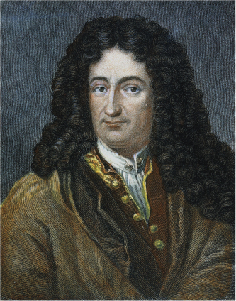
The “prime” notation y′ and f′(x) was introduced by the French mathematician Joseph Louis Lagrange (1736–1813). There is another standard notation for the derivative that we owe to Leibniz (Figure 2):
In Example 2, we showed that the derivative of y = x−2 is y′ = −2x−3. In Leibniz notation, we would write
To specify the value of the derivative for a fixed value of x, say, x = 4, we write
Thinking of \(\frac{dy}{dx}\) as a fraction forces us to confront the question: what actually are \(dy\) and \(dx\) ? We cannot answer this question precisely. Leibniz thought of them as "infinitely small" changes in \(y\) and \(x\) . The notation, however, proved to be so incredibly useful (especially to physicists) that in the first half of the 20th century mathematicians figured out a rigorous explanation which is now known as the theory of differential forms which you may encounter in your advanced studies.
CONCEPTUAL INSIGHT
Leibniz notation is widely used for several reasons. First, it reminds us that the derivative df/dx, although not itself a ratio, is in fact a limit of ratiosΔf/Δx. Second, the notation specifies the independent variable. This is useful when variables other than x are used. For example, if the independent variable is t, we write df/dt. Third, we often think of d/dx as an “operator” that performs differentiation on functions. In other words, we apply the operator d/dx to f to obtain the derivative df/dx. We will see other advantages of Leibniz notation when we discuss the Chain Rule in Section 3.7.
A main goal of this chapter is to develop the basic rules of differentiation. These rules enable us to find derivatives without computing limits.
131
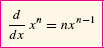
The Power Rule is valid for all exponents. We prove it here for a whole number n (see Exercise 95 for a negative integer n and p. 183 for arbitrary n).
THEOREM 1 The Power Rule
For all exponents n,
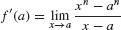
Proof
Assume that n is a whole number and let f(x) = xn. Then
To simplify the difference quotient, we need to generalize the following identities:
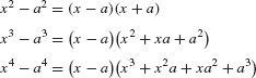
The generalization is

To verify Eq. (2), observe that the right-hand side is equal to
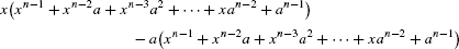
When we carry out the multiplications, all terms cancel except the first and the last, so only xn − an remains, as required.
Equation (2) gives us

Therefore,
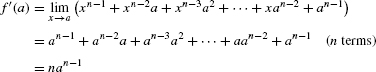
This proves that f′(a) = nan−1, which we may also write as f′(x) = nxn−1.
Question 1.4 Derivative As a Function Progress Check 2
Find \(\frac{dy}{dx}\) for \(y=x^{17}\)
| A. |
| B. |
| C. |
CAUTION The Power Rule applies only to the power functions y = xn. It does not apply to exponential functions such as \(y=2^x\). The derivative of \(y=2^x\)is not \(x 2^{x-1}\). We will study the derivatives of exponential functions later in this section.
We make a few remarks before proceeding:
- It may be helpful to remember the Power Rule in words: To differentiate xn, “bring down the exponent and subtract one (from the exponent).”
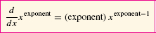
- • The Power Rule is valid for all exponents, whether negative, fractional, or irrational:
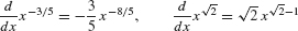
132
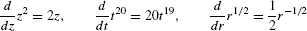
- The Power Rule can be applied with any variable, not just x. For example,
Next, we state the Linearity Rules for derivatives, which are analogous to the linearity laws for limits.
THEOREM 2 Linearity Rules
Assume that f and g are differentiable. Then
Sum and Difference Rules:f + g and f − g are differentiable, and
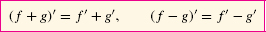
or, in Leibniz notation,
\(\Large \frac{d}{dx} (f(x) + g(x))= \frac{d}{dx} f(x) + \frac{d}{dx} g(x)\)
and
\(\Large \frac{d}{dx} (f(x) - g(x))= \frac{d}{dx} f(x) - \frac{d}{dx} g(x)\)
Constant Multiple Rule: For any constant c, cf is differentiable and

or, in Leibniz notation,
\(\frac{d}{dx} (cf(x) )=c \frac{d}{dx} f(x)\)
Proof
To prove the Sum Rule, we use the definition

This difference quotient is equal to a sum (h ≠ 0):

Therefore, by the Sum Law for limits,
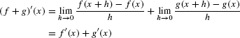
as claimed. The Difference and Constant Multiple Rules are proved similarly.
EXAMPLE 3
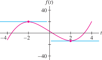
Find the points on the graph of f(t) = t3 − 12t + 4 where the tangent line is horizontal (Figure 3).
Solution We calculate the derivative:
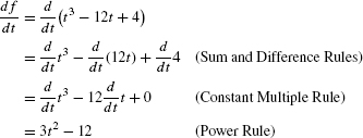
Note in the second line that the derivative of the constant 4 is zero. The tangent line is horizontal at points where the slope f′(t) is zero, so we solve

Now f(2) = −12 and f(−2) = 20. Hence, the tangent lines are horizontal at (2, −12) and (−2, 20).
133
EXAMPLE 4
Calculate  , where
 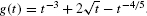 .
.
Solution We differentiate term-by-term using the Power Rule without justifying the intermediate steps. Writing  , we have
Question 1.5 Derivative As a Function Progress Check 3
Find the derivative \(f'(-1)\) for \(f(t)= 5t^3+2t^2-1\)
The derivative f′(x) gives us important information about the graph of f(x). For example, the sign of f′(x) tells us whether the tangent line has positive or negative slope, and the magnitude of f′(x) reveals how steep the slope is.
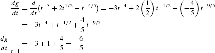
EXAMPLE 5 Graphical Insight
How is the graph of f(x) = x3 − 12x2 + 36x − 16 related to the derivative f′(x) = 3x2 − 24x + 36?
Solution The derivative f′(x) = 3x2 − 24x + 36 = 3(x − 6)(x− 2) is negative for 2 < x < 6 and positive elsewhere [Fig. 4(B)]. The following table summarizes this sign information[Fig. 4(A)]:
| Property of f′(x) | Property of the Graph of f (x) |
|---|---|
| f′(x) < 0 for 2 < x < 6 | Tangent line has negative slope for 2 < x < 6. |
| f′(2) = f′(6) = 0 | Tangent line is horizontal at x = 2 and x = 6. |
| f′(x) > 0 for x < 2 and x > 6 | Tangent line has positive slope for x < 2 and x > 6. |
Note also that f′(x) → ∞ as |x| becomes large. This corresponds to the fact that the tangent lines to the graph of f(x) get steeper as |x| grows large.
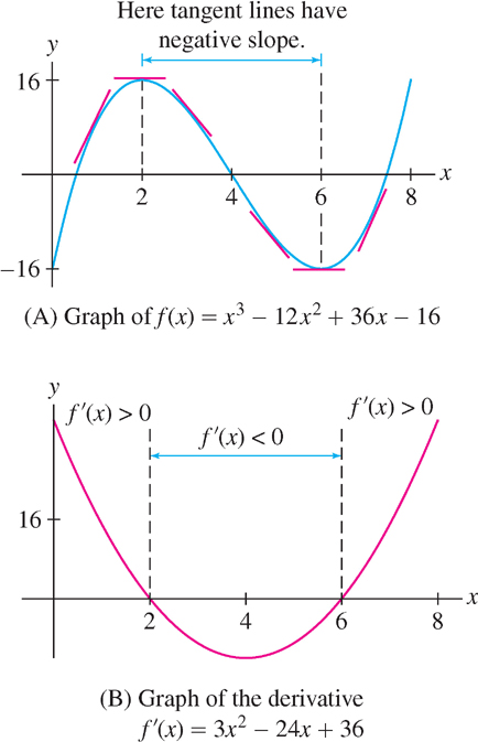
EXAMPLE 6 Identifying the Derivative
The graph of f(x) is shown in Figure 5(A). Which graph (B) or (C), is the graph of f′(x)?
| Slope of Tangent Line | Where |
|---|---|
| Negative | (0, 1) and (4, 7) |
| Zero | x = 1, 4, 7 |
| Positive | (1, 4) and (7, ∞) |
Solution In Figure 5(A) we see that the tangent lines to the graph have negative slope on the intervals (0, 1) and (4, 7). Therefore f′(x) is negative on these intervals. Similarly (see the table in the margin), the tangent lines have positive slope (and f′(x) is positive) on the intervals (1, 4) and (7, ∞). Only (C) has these properties, so (C) is the graph of f′(x).
134
1.6 Question Demos - Embedded Queries etc.
Advanced question setups: Google It.
Question 1.6
This is a fill-in-the- query. This is a query.
Dynamic Figure test.
Question 1.7
What is the capital of Oregon?
| A. |
| B. |
| C. |
1.7 Video Link to UC Brightcove Video Test
Here is a Brightcove video link.