10.1 Sequences
Sequences of numbers appear in diverse situations. If you divide a cake in half, and then divide the remaining half in half, and continue dividing in half indefinitely (Figure 10.1), then the fraction of cake remaining at each step forms the sequence \[ 1,\quad \frac12, \quad \frac14,\quad \frac18,\quad \dots \] This is the sequence of values of the function \(f(n)=\frac1{2^n}\) for \(n=0,1,2,\dots.\)
Formally, a sequence is an ordered collection of numbers defined by a function \(f(n)\) on a set of integers. The values \(a_n=f(n)\) are called the terms of the sequence, and \(n\) is called the index. Informally, we think of a sequence \(\{a_n\}\) as a list of terms: \[ a_1,\quad a_2,\quad a_3, \quad a_4, \quad\dots \] The sequence does not have to start at \(n=1\), but may start at \(n=0\), \(n=2\), or any other integer. When \(a_n\) is given by a formula, we refer to \(a_n\) as the general term.

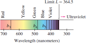
The sequence \(b_n\) is the Balmer series of absorption wavelengths of the hydrogen atom in nanometers. It plays a key role in spectroscopy.
| General term | Domain | Sequence |
| \(a_n = 1-\dfrac{1}{n}\) | \(n\ge 1\) | \(0,\,\, \dfrac12,\,\, \dfrac23,\,\,\dfrac34,\,\, \dfrac45,\,\,\dots\) |
| \(a_n = (-1)^{n}n\) | \(n\ge 0\) | \(0,\,\, -1,\,\, 2, \,\,-3,\,\, 4,\,\,\dots\) |
| \(b_n = \dfrac{364.5n^2}{n^2-4}\) | \(n\ge 3\) | \(656.1, \,\, 486,\,\, 433.9,\,\, 410.1,\,\, 396.9,\,\, \dots\) |
The sequence in the next example is defined recursively. The first term is given and the \(n\)th term \(a_n\) is computed in terms of the preceding term \(a_{n-1}\).
538
EXAMPLE 1 Recursive Sequence
Compute \(a_2, a_3, a_4\) for the sequence defined recursively by \[ a_1 = 1,\qquad a_n = \frac12\left(a_{n-1}+\frac2{a_{n-1}}\right) \]
Solution
\[ \begin{alignat*}{2} a_2 = \frac12\left(a_1+\frac2{a_1}\right)~= \frac12\left(1+\frac2{1}\right) &~= \frac32 = 1.5\\ a_3 = \frac12\left(a_2+\frac2{a_2}\right) = \frac12\left(\frac32+\frac2{3/2}\right)~ &= \frac{17}{12}\approx 1.4167\\ a_4 =\; \frac12\left(a_3+\frac2{a_3}\right) = \frac12\left(\frac{17}{12}+\frac2{17/12}\right)~ &= \frac{577}{408}\approx 1.414216 \end{alignat*} \]
You may recognize the sequence in Example 1 as the sequence of approximations to \(\sqrt 2\approx 1.4142136\) produced by Newton’s method with starting value \(a_1=1\). As \(n\) tends to infinity, \(a_n\) approaches \(\sqrt 2\).
Our main goal is to study convergence of sequences. A sequence \(\{a_n\}\) converges to a limit \(L\) if \(|a_n-L|\) becomes arbitrary small when \(n\) is sufficiently large. Here is the formal definition.
DEFINITION Limit of a Sequence
We say that \(\{a_n\}\) converges to a limit \(L\), and we write \[ \lim_{n\to\infty} a_n = L\qquad\textrm{or}\qquad a_n\to L \] if, for every \(\epsilon >0\), there is a number \(M\) such that \(|a_n-L|<\epsilon\) for all \(n > M\).
- If no limit exists, we say that \(\{a_n\}\) diverges.
- If the terms increase without bound, we say that \(\{a_n\}\) diverges to infinity.
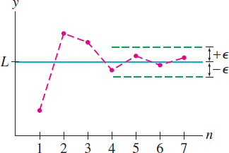
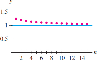
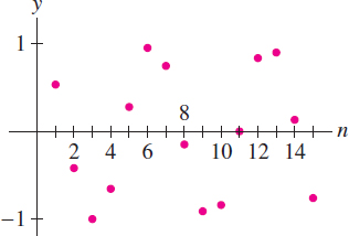
If \(\{a_n\}\) converges, then its limit \(L\) is unique. A good way to visualize the limit is to plot the points \((1, a_1), (2, a_2), (3, a_3), \dots\), as in Figure 10.2. The sequence converges to \(L\) if, for every \(\epsilon>0\), the plotted points eventually remain within an \(\epsilon\)-band around the horizontal line \(y=L\). Figure 10.3 shows the plot of a sequence converging to \(L=1\). On the other hand, we can show that the sequence \(a_n=\cos n\) in Figure 10.4 has no limit.
EXAMPLE 2 Proving Convergence
Let \(a_n\! =\! \frac{n+4}{n+1}\). Prove formally that \( \displaystyle\lim_{n\to\infty} a_n\! =\! 1\).
Solution The definition requires us to find, for every \(\epsilon>0\), a number \(M\) such that \[ \begin{equation*} |a_n - 1|<\epsilon \qquad\textrm{for all \(n>M\)}\tag{1} \end{equation*} \]
539
We have \[ |a_n-1|~=\Bigg|\frac{n+4}{n+1} - 1\Bigg|~= \frac3{n+1} \] Therefore, \(|a_n-1|<\epsilon\) if \[ \frac3{n+1} < \epsilon \qquad\textrm{or}\qquad n >\frac{3}{\epsilon}-1 \] In other words, Eq. (1) is valid with \(M = \tfrac{3}{\epsilon}-1\). This proves that \(\lim\limits_{n\to\infty} a_n = 1\).
Note the following two facts about sequences:
- The limit does not change if we change or drop finitely many terms of the sequence.
- If \(C\) is a constant and \(a_n =C\) for all \(n\) sufficiently large, then \(\lim\limits_{n\to\infty}a_n=C\).
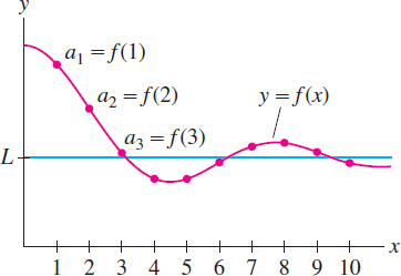
Many of the sequences we consider are defined by functions; that is, \(a_n = f(n)\) for some function \(f(x)\). For example, \[ a_n=\frac{n-1}n \qquad\textrm{is defined by}\qquad f(x)=\frac{x-1}x \] A fact we will use often is that if \(f(x)\) approaches a limit \(L\) as \(x\to\infty\), then the sequence \(a_n = f(n)\) approaches the same limit \(L\) (Figure 10.5). Indeed, for all \(\epsilon>0\), we can find \(M\) so that \(|f(x)-L|<\epsilon\) for all \(x>M\). It follows automatically that \(|f(n)-L|<\epsilon\) for all integers \(n>M\).
THEOREM 1 Sequence Defined by a Function
If \(\lim\limits_{x\to\infty}f(x)\) exists, then the sequence \(a_n = f(n)\) converges to the same limit: \[ \lim\limits_{n\to\infty} a_n = \lim\limits_{x\to\infty}f(x) \]
EXAMPLE 3
Find the limit of the sequence \[ \dfrac{2^2-2}{2^2},\quad \dfrac{3^2-2}{3^2},\quad \dfrac{4^2-2}{4^2},\quad \dfrac{5^2-2}{5^2},\quad \dots \]
Solution This is the sequence with general term \[ a_n=\frac{n^2-2}{n^2} = 1 - \frac2{n} \] Therefore, we apply Theorem 1 with \(f(x)=1-\tfrac{2}{x}\): \[ \lim\limits_{n\to\infty} a_n =\lim\limits_{x\to\infty} \left(1-\frac2{x}\right)=1-\lim\limits_{x\to\infty}\frac2{x}=1 - 0 = 1 \]
EXAMPLE 4
Calculate \(\lim\limits_{n\to\infty} \frac{n+\ln n}{n^2}\).
Solution Apply Theorem 1, using L'Hôpital’s Rule in the second step: \[ \lim\limits_{n\to\infty}\frac{n+\ln n}{n^2} = \lim\limits_{x\to\infty}\frac{x+\ln x}{x^2} = \lim\limits_{x\to\infty}\frac{1+(1/x)}{2x} = 0 \]
540
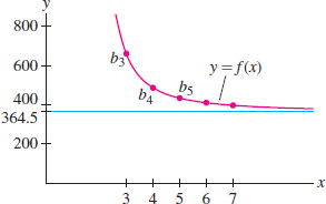
The limit of the Balmer wavelengths \(b_n\) in the next example plays a role in physics and chemistry because it determines the ionization energy of the hydrogen atom. Table 10.1 suggests that \(b_n\) approaches \(364.5\). Figure 10.6 shows the graph, and in Figure 10.7, the wavelengths are shown “crowding in” toward their limiting value.
| \(n\) | \(b_n\) |
|---|---|
| 3 | 656.1 |
| 4 | 486 |
| 5 | 433.9 |
| 6 | 410.1 |
| 7 | 396.9 |
| 10 | 379.7 |
| 20 | 368.2 |
| 40 | 365.4 |
| 60 | 364.9 |
| 80 | 364.7 |
| 100 | 364.6 |
EXAMPLE 5 Balmer Wavelengths
Calculate the limit of the Balmer wavelengths \(b_n= \frac{364.5n^2}{n^2-4}\), where \(n \geq 3\).
Solution Apply Theorem 1 with \(f(x)= \frac{364.5x^2}{x^2-4}\): \[ \lim\limits_{n\to\infty}b_n = \lim\limits_{x\to\infty}\frac{364.5x^2}{x^2-4} = \lim\limits_{x\to\infty}\frac{364.5}{1-4/x^2} =\dfrac{364.5}{\lim\limits_{x\to\infty}(1-4/x^2)} = 364.5 \]
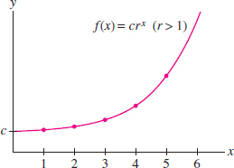
A geometric sequence is a sequence \(a_n=cr^n\), where \(c\) and \(r\) are nonzero constants. Each term is \(r\) times the previous term; that is, \(a_n/a_{n-1}=r\). The number \(r\) is called the common ratio. For instance, if \(r=3\) and \(c=2\), we obtain the sequence (starting at \(n=0\)) \[ 2,\quad 2\cdot 3,\quad 2\cdot 3^2,\quad 2\cdot 3^3,\quad 2\cdot 3^4,\quad 2\cdot 3^5,\quad\dots \] In the next example, we determine when a geometric series converges. Recall that \(\{a_n\}\) diverges to \(\infty\) if the terms \(a_n\) increase beyond all bounds (Figure 10.8); that is, \[ \lim\limits_{n\to\infty}a_n=\infty\quad\textrm{if, for every number}\;N, a_n>N \textrm{for all sufficiently large}\;n \] We define \(\lim\limits_{n\to\infty}a_n= - \infty\) similarly.
EXAMPLE 6 Geometric Sequences with \(r \geq 0\)
Prove that for \(r\ge 0\) and \(c>0\), \[\begin{align*} \lim\limits_{n\to\infty}cr^n = \begin{cases} 0 & \text{if}\quad 0\le r <1\\ c & \text{if}\quad r=1\\ \infty & \text{if}\quad r > 1 \end{cases} \end {align*}\]
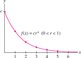
Solution Set \(f(r)=cr^x\). If \(0\le r<1\), then (Figure 10.9) \[ \lim\limits_{n\to\infty}cr^n = \lim\limits_{x\to\infty}f(x) = c\lim\limits_{x\to\infty}r^x = 0 \]
If \(r>1\), then both \(f(x)\) and the sequence \(\{cr^n\}\) diverge to \(\infty\) (because \(c>0\)) (Figure 10.8).
If \(r=1\), then \(cr^n=c\) for all \(n\), and the limit is \(c\).
541
The limit laws we have used for functions also apply to sequences and are proved in a similar fashion.
THEOREM 2 Limit Laws for Sequences
Assume that \(\{a_n\}\) and \(\{b_n\}\) are convergent sequences with \[ \lim\limits_{n\to\infty}a_n = L,\qquad \lim\limits_{n\to\infty}b_n = M \]
Then:
- \(\lim\limits_{n\to\infty}(a_n\pm b_n) = \lim\limits_{n\to\infty} a_n \pm\lim\limits_{n\to\infty} b_n = L\pm M\)
- \(\lim\limits_{n\to\infty} a_nb_n = \Big(\lim\limits_{n\to\infty}a_n\Big)\Big(\lim\limits_{n\to\infty}b_n\Big) = LM\)
- \(\lim\limits_{n\to\infty}\frac{a_n}{b_n} = \frac{\lim\limits_{n\to\infty}a_n}{ \lim\limits_{n\to\infty}b_n} = \frac{L}M \textrm{if}~M \ne 0\)
- \(\lim\limits_{n\to\infty} ca_n = c\lim\limits_{n\to\infty}a_n = cL\) for any constant \(c\)
THEOREM 3 Squeeze Theorem for Sequences
Let \(\{a_n\}\), \(\{b_n\}\), \(\{c_n\}\) be sequences such that for some number \(M\), \[ b_n\le a_n\le c_n\quad\textrm{for \(n>M\)}\qquad\textrm{and}\qquad \lim\limits_{n\to\infty}b_n = \lim\limits_{n\to\infty}c_n = L \] Then \(\lim\limits_{n\to\infty}a_n = L\).
Reminder
\(n!\)(\(n\)-factorial) is the number \[ n! = n(n-1)(n-2)\cdots 2\cdot 1 \] For example, \(4!=4\cdot 3\cdot 2\cdot 1 = 24\).
EXAMPLE 7
Show that if \(\lim\limits_{n\to\infty}|a_n|=0\), then \(\lim\limits_{n\to\infty}a_n=0\).
Solution We have \[ -|a_n|\le a_n \le |a_n| \] By hypothesis, \(\lim\limits_{n\to\infty} |a_n| = 0\), and thus also \(\lim\limits_{n\to\infty}-|a_n| =-\lim\limits_{n\to\infty}|a_n|=0\). Therefore, we can apply the Squeeze Theorem to conclude that \(\lim\limits_{n\to\infty}a_n=0\).
EXAMPLE 8 Geometric Sequences with \(r<0\)
Prove that for \(c\ne 0\), \[ \lim\limits_{n\to\infty}cr^n = \begin{cases} 0 & \text{if}\quad -1< r < 0\\ \textrm{diverges} & \text{if} \quad r \le -1 \end{cases} \]
Solution If \(-1< r < 0\), then \(0<|r|<1\) and \(\lim\limits_{n\to\infty}|cr^n|=0\) by Example 6. Thus \(\lim\limits_{n\to\infty}cr^n=0\) by Example 7. If \(r= -1\), then the sequence \(cr^{n} = (-1)^nc\) alternates in sign and does not approach a limit. The sequence also diverges if \(r<-1\) because \(cr^n\) alternates in sign and \(|cr^{n}|\) grows arbitrarily large.
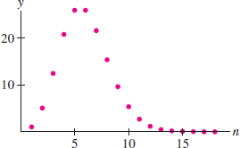
As another application of the Squeeze Theorem, consider the sequence \[ a_n=\frac{5^n}{n!} \] Both the numerator and the denominator grow without bound, so it is not clear in advance whether \(\{a_n\}\) converges. Figure 10.10 and Table suggest that \(a_n\) increases initially and then tends to zero. In the next example, we verify that \(a_n={R^n}/{n!}\) converges to zero for all \(R\). This fact centering is used in the discussion of Taylor series in Section 10.7.
| (n) | \(a_n=\frac{5^n}{n!}\) |
| 1 | 5 |
| 2 | 12.5 |
| 3 | 20.83 |
| 4 | 26.04 |
| 10 | 2.69 |
| 15 | 0.023 |
| 20 | 0.000039 |
| 50 | 2.92\(\times 10^{-30}\) |
542
EXAMPLE 9
Prove that \(\lim\limits_{n\to\infty}\frac{R^n}{n!} = 0\) for all \(R\).
Solution Assume first that \(R>0\) and let \(M\) be the positive integer such that \[ M\le R < M+1 \] For \(n>M\), we write \(R^n/n!\) as a product of \(n\) factors: \[ \begin{equation*} \frac{R^n}{n!} = \underbrace{\left(\frac{R}{1}\frac{R}{2}\cdots\frac{R}{M}\right)} _{\textrm{Call this constant \(C\)}} \underbrace{\left(\frac{R}{M+1}\right)\left(\frac{R}{M+2}\right) \cdots\left(\frac{R}{n}\right)}_{\textrm{Each factor is less than 1}} \le C\left(\frac{R}{n}\right)\tag{2} \end{equation*} \] The first \(M\) factors are \(\ge 1\) and the last \(n-M\) factors are \(<1\). If we lump together the first \(M\) factors and call the product \(C\), and drop all the remaining factors except the last factor \(R/n\), we see that \[ 0\le \frac{R^n}{n!}\le \frac{CR}{n} \] Since \({CR}/{n}\to 0\), the Squeeze Theorem gives us \(\lim\limits_{n\to\infty}{R^n}/{n!} = 0\) as claimed. If \(R<0\), the limit is also zero by Example 7 because \(\left|{R^n}/{n!}\right|\) tends to zero.
Given a sequence \(\{a_n\}\) and a function \(f(x)\), we can form the new sequence \(f(a_n)\). It is useful to know that if \(f(x)\) is continuous and \(a_n\to L\), then \(f(a_n) \to f(L)\). A proof is given in Appendix D.
THEOREM 4
If \(f(x)\) is continuous and \(\lim\limits_{n\to\infty} a_n = L\), then \[ \lim\limits_{n\to\infty}f(a_n) = f\Bigl(\lim\limits_{n\to\infty}a_n\Bigr) = f(L) \] In other words, we may “bring a limit inside a continuous function.”
EXAMPLE 10
Apply Theorem 4 to the sequence \(a_n = \frac{3n}{n+1}\) and to the functions
(a) \(f(x) = e^x\) and (b) \(g(x) = x^2\).
Solution Observe first that \[ L = \lim\limits_{n\to\infty}a_n = \lim\limits_{n\to\infty} \frac{3n}{n+1} = \lim\limits_{n\to\infty} \frac{3}{1+n^{-1}} = 3 \]
- With \(f(x)=e^x\) we have \( f(a_n) = e^{a_n} = e^{\frac{3n}{n+1}}\). According to Theorem 4, \[ \lim\limits_{n\to\infty} e^{\frac{3n}{n+1}} =\lim\limits_{n\to\infty} f(a_n) = f\Bigl(\lim\limits_{n\to\infty} a_n\Bigr) = e^{\mkern1mu\lim\limits_{n\to\infty} \frac{3n}{n+1}} = e^3 \]
- With \(g(x)=x^2\) we have \(g(a_n)=a_n^2\), and according to Theorem 4, \[ \lim\limits_{n\to\infty} \left(\frac{3n}{n+1}\right)^2 =\lim\limits_{n\to\infty} g(a_n) = g\Bigl(\lim\limits_{n\to\infty} a_n\Bigr) = \left(\lim\limits_{n\to\infty} \frac{3n}{n+1}\right)^2 = 3^2 = 9 \]
Of great importance for understanding convergence are the concepts of a bounded sequence and a monotonic sequence.
543
DEFINITION Bounded Sequences
A sequence \(\{a_n\}\) is:
- Bounded from above if there is a number \(M\) such that \(a_n\le M\) for all \(n\). The number \(M\) is called an upper bound.
- Bounded from below if there is a number \(m\) such that \(a_n\ge m\) for all \(n\). The number \(m\) is called a lower bound.
The sequence \(\{a_n\}\) is called bounded if it is bounded from above and below. A sequence that is not bounded is called an unbounded sequence.
Upper and lower bounds are not unique. If \(M\) is an upper bound, then any larger number is also an upper bound, and if \(m\) is a lower bound, then any smaller number is also a lower bound (Figure 10.11).
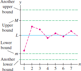
As we might expect, a convergent sequence \(\{a_n\}\) is necessarily bounded because the terms \(a_n\) get closer and closer to the limit. This fact is recorded in the next theorem.
THEOREM 5 Convergent Sequences Are Bounded
If \(\{a_n\}\) converges, then \(\{a_n\}\) is bounded.
Proof
Let \(L=\lim\limits_{n\to\infty}a_n\). Then there exists \(N>0\) such that \(|a_n - L|<1\) for \(n>N\). In other words, \[ L-1<a_n<L+1\qquad\textrm{for \(n>N\)} \] If \(M\) is any number larger than \(L+1\) and also larger than the numbers \(a_1, a_2, \dots, a_N\), then \(a_n<M\) for all \(n\). Thus, \(M\) is an upper bound. Similarly, any number \(m\) smaller than \(L-1\) and also smaller than the numbers \(a_1, a_2, \dots, a_N\) is a lower bound.
There are two ways that a sequence \(\{a_n\}\) can diverge. One way is by being unbounded. For example, the unbounded sequence \(a_n = n\) diverges: \[ 1,\quad 2,\quad 3,\quad 4,\quad 5,\quad 6,\quad \dots \] However, a sequence can diverge even if it is bounded. This is the case with \(a_n = (-1)^{n+1}\), whose terms \(a_n\) bounce back and forth but never settle down to approach a limit: \[ 1,\quad -1,\quad 1,\quad -1,\quad 1,\quad -1,\quad \dots \]
There is no surefire method for determining whether a sequence \(\{a_n\}\) converges, unless the sequence happens to be both bounded and monotonic. By definition, \(\{a_n\}\) is monotonic if it is either increasing or decreasing:
- \(\{a_n\}\) is increasing if \(a_n < a_{n+1}\) for all \(n\).
- \(\{a_n\}\) is decreasing if \(a_n > a_{n+1}\) for all \(n\).
Intuitively, if \(\{a_n\}\) is increasing and bounded above by \(M\), then the terms must bunch up near some limiting value \(L\) that is not greater than \(M\) (Figure 10.12. See Appendix B for a proof of the next theorem.

544
THEOREM 6 Bounded Monotonic Sequences Converge
- If \(\{a_n\}\) is increasing and \(a_n\le M\), then \(\{a_n\}\) converges and \(\lim\limits_{n\to\infty} a_n \le M\).
- If \(\{a_n\}\) is decreasing and \(a_n\ge m\), then \(\{a_n\}\) converges and \(\lim\limits_{n\to\infty} a_n \ge m\).
EXAMPLE 11
Verify that \(a_n=\sqrt{n+1}-\sqrt n\) is decreasing and bounded below. Does \(\lim\limits_{n\to\infty}a_n\) exist?
| \(a_n=\sqrt{n+1}-\sqrt{n}\) |
| \(a_1 \approx 0.4142\) |
| \(a_2 \approx 0.3178\) |
| \(a_3 \approx 0.2679\) |
| \(a_4 \approx 0.2361\) |
| \(a_5 \approx 0.2134\) |
| \(a_6 \approx 0.1963\) |
| \(a_7 \approx 0.1827\) |
| \(a_8 \approx 0.1716\) |
Solution The function \(f(x)=\sqrt{x+1}-\sqrt x\) is decreasing because its derivative is negative: \[ f'(x) = \frac1{2\sqrt{x+1}} - \frac1{2\sqrt{x}} < 0 \qquad\textrm{for \(x>0\)} \] It follows that \(a_n = f(n)\) is decreasing (see Table ). Furthermore, \(a_n > 0\) for all \(n\), so the sequence has lower bound \(m=0\). Theorem 6 guarantees that \(L=\lim\limits_{n\to\infty}a_n\) exists and \(L\ge 0\). In fact, we can show that \(L=0\) by noting that \(f(x) = 1/(\sqrt{x+1}+\sqrt x)\) and hence \(\lim\limits_{x\to\infty}f(x)=0\).
EXAMPLE 12
Show that the following sequence is bounded and increasing: \[ a_1=\sqrt{2},\quad a_2=\sqrt{2\sqrt{2}},\quad a_3=\sqrt{2\sqrt{2\sqrt{2}}},\quad \dots\quad \] Then prove that \(L=\lim\limits_{n\to\infty}a_n\) exists and compute its value.
Solution If we knew in advance that the limit \(L\) exists, we could find its value as follows. The idea is that \(L\) “contains a copy” of itself under the square root sign: \[ L = \sqrt{2\sqrt{2\sqrt{2\sqrt{2\cdots }}}} = \sqrt{2\left(\sqrt{2\sqrt{2\sqrt{2\cdots }}}\right)} = \sqrt{2L} \] Thus \(L^2=2L\), which implies that \(L = 2\) or \(L=0\). We eliminate \(L=0\) because the terms \(a_n\) are positive and increasing (as shown below), so we must have \(L=2\) (see Table ).
This argument is phrased more formally by noting that the sequence is defined recursively by \[ a_1=\sqrt{2},\qquad a_{n+1}=\sqrt{2a_n} \] If \(a_n\) converges to \(L\), then the sequence \(b_n = a_{n+1}\) also converges to \(L\) (because it is the same sequence, with terms shifted one to the left). Then, using Theorem 4, we would have \[ L = \lim\limits_{n\to\infty} a_{n+1} = \lim\limits_{n\to\infty} \sqrt{2a_n} =\sqrt{2\lim\limits_{n\to\infty}a_n}=\sqrt{2L} \] However, none of this is valid unless we know in advance that the limit \(L\) exists. By Theorem 6, it suffices to show that \(\{a_n\}\) is bounded above and increasing.
| \(a_1\) | \(1.4142\) |
| \(a_2\) | \(1.6818\) |
| \(a_3\) | \(1.8340\) |
| \(a_4\) | \(1.9152\) |
| \(a_5\) | \(1.9571\) |
| \(a_6\) | \(1.9785\) |
| \(a_7\) | \(1.9892\) |
| \(a_8\) | \(1.9946\) |
Step 1. Show that \(\{a_n\}\) is bounded above.
We claim that \(M=2\) is an upper bound. We certainly have \(a_1 < 2\) because \(a_1=\sqrt{2}\approx 1.414\). On the other hand, \[ \begin{equation*} {if} a_n<2,\qquad {then}\qquad a_{n+1} < 2\tag{3} \end{equation*} \]
545
This is true because \(a_{n+1}=\sqrt{2a_n}<\sqrt{2\cdot 2}=2\). Now, since \(a_1 < 2\), we can apply (3) to conclude that \(a_2<2\). Similarly, \(a_2<2\) implies \(a_3<2\), and so on for all \(n\). Formally speaking, this is a proof by induction.
Step 2. Show that \(\{a_n\}\) is increasing
Since \(a_n\) is positive and \(a_n < 2\), we have \[ a_{n+1} = \sqrt{2a_n}> \sqrt{a_n\cdot a_n} = a_n \] This shows that \(\{a_n\}\) is increasing.
We conclude that the limit \(L\) exists and hence \(L=2\).
10.1.1 Summary
- A sequence \(\{a_n\}\) converges to a limit \(L\) if, for every \(\epsilon >0\), there is a number \(M\) such that \[ |a_n-L|<\epsilon \qquad\textrm{for all \(n>M\)} \] We write \(\lim\limits_{n\to\infty}a_n=L\) or \(a_n\to L\).
- If no limit exists, we say that \(\{a_n\}\) diverges.
- In particular, if the terms increase without bound, we say that \(\{a_n\}\) diverges to infinity.
- If \(a_n=f(n)\) and \(\lim\limits_{x\to \infty} f(x) = L\), then \(\lim\limits_{n\to\infty}a_n=L\).
- A geometric sequence is a sequence \(a_n=cr^n\), where \(c\) and \(r\) are nonzero.
- The Basic Limit Laws and the Squeeze Theorem apply to sequences.
- If \(f(x)\) is continuous and \(\lim\limits_{n\to\infty}a_n=L\), then \(\lim\limits_{n\to\infty}f(a_n)=f(L)\).
- A sequence \(\{a_n\}\) is
- - bounded above by \(M\) if \(a_n\leq M\) for all \(n\).
- - bounded below by \(m\) if \(a_n\geq m\) for all \(n\).
If \(\{a_n\}\) is bounded above and below, \(\{a_n\}\) is called bounded.
- A sequence \(\{a_n\}\) is monotonic if it is increasing (\(a_n< a_{n+1}\)) or decreasing (\(a_n > a_{n+1})\).
- Bounded monotonic sequences converge (Theorem 6).