14.1 Functions of Two or More Variables
A familiar example of a function of two variables is the area \(A\) of a rectangle, equal to the product \(xy\) of the base \(x\) and height \(y\). We write \[ A(x,y) = xy \] or \(A =f(x,y)\), where \(f(x,y) = xy\). An example in three variables is the distance from a point \(P=(x,y,z)\) to the origin: \[ g(x,y,z) = \sqrt{x^2+y^2+z^2} \]
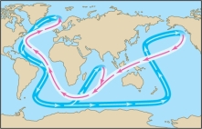
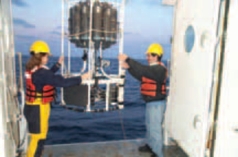
An important but less familiar example is the density of seawater, denoted \(\rho\), which is a function \(\rho(S,T)\) of salinity \(S\) and temperature \(T\) (Figure 14.1). Although there is no simple formula for \(\rho(S,T)\), scientists determine function values experimentally (Figure 14.2). According to Table 14.1, if \(S=32\) (in parts per thousand) and \(T=10^\circ\)C, then \[ \rho(32,10) = 1.0246~\text{kg/m}^3 \]
| Salinity (ppt) | |||
|---|---|---|---|
| \(^\circ\mathrm{C}\) | \(32\) | \(32.5\) | \(33\) |
| \(~5\) | \(1.0253\) | \(1.0257\) | \(1.0261\) |
| \(10\) | \(1.0246\) | \(1.0250\) | \(1.0254\) |
| \(15\) | \(1.0237\) | \(1.0240\) | \(1.0244\) |
| \(20\) | \(1.0224\) | \(1.0229\) | \(1.0232\) |
A function of \(n\) variables is a function \(f(x_1,\dots,x_n)\) that assigns a real number to each \(n\)-tuple \((x_1,\dots,x_n)\) in a domain in \({\bf{R}}^n\). Sometimes we write \(f(P)\) for the value of \(f\) at a point \(P = (x_1, \ldots, x_n)\). When \(f\) is defined by a formula, we usually take as domain the set of all \(n\)-tuples for which \(f(x_1,\dots,x_n)\) is defined. The range of \(f\) is the set of all values \(f(x_1,\dots,x_n)\) for \((x_1,\dots,x_n)\) in the domain. Since we focus on functions of two or three variables, we shall often use the variables \(x,y\), and \(z\) (rather than \(x_1, x_2\), \(x_3\)).
775
EXAMPLE 1
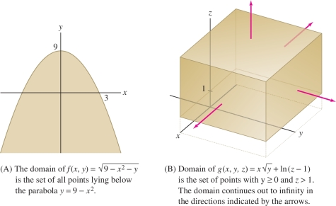
Sketch the domains of
- (a) \(f(x,y) = \sqrt{9-x^2-y}\)
- (b) \(g(x,y,z) = x\sqrt{y}+\ln (z-1)\)
What are the ranges of these functions?
Solution (a) \(f(x,y) = \sqrt{9- x^2-y}\) is defined only when \(9- x^2-y\ge 0\), or \(y \le 9-x^2\). Thus the domain consists of all points \((x,y)\) lying below the parabola \(y=9-x^2\) [Figure 14.3]: \[ {\mathcal{D}}=\{(x,y): y\le 9-x^2\} \]
To determine the range, note that \(f\) is a nonnegative function and that \(f(0,y)=\sqrt{9-y}\). Since \(9-y\) can be any positive number, \(f(0,y)\) takes on all nonnegative values. Therefore the range of \(f\) is the infinite interval \([0,\infty)\).
(b) \(g(x,y,z) = x\sqrt{y}+\ln (z-1)\) is defined only when both \(\sqrt y\) and \(\ln (z - 1)\) are defined. We must require that \(y \geq 0\) and \(z > 1\), so the domain is \(\{(x,y,z): y\ge 0, z>1\}\) [Figure 14.3]. The range of \(g\) is the entire real line \({\bf{R}}\). Indeed, for the particular choices \(y=1\) and \(z=2\), we have \(g(x,1,2)=x\sqrt{1}+\ln 1 = x\), and since \(x\) is arbitrary, we see that \(g\) takes on all values.
Graphing Functions of Two Variables
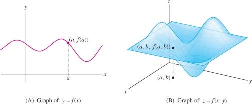
In single-variable calculus, we use graphs to visualize the important features of a function. Graphs play a similar role for functions of two variables. The graph of \(f(x,y)\) consists of all points \((a,b,f(a,b))\) in \({\bf{R}}^3\) for \((a,b)\) in the domain \({\mathcal{D}}\) of \(f\). Assuming that \(f\) is continuous (as defined in the next section), the graph is a surface whose height above or below the \(xy\)-plane at \((a,b)\) is the function value \(f(a,b)\) [Figure 14.4]. We often write \(z=f(x,y)\) to stress that the \(z\)-coordinate of a point on the graph is a function of \(x\) and \(y\).
EXAMPLE 2
Sketch the graph of \(f(x,y)= 2x^2+5y^2\).
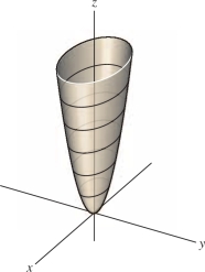
Solution The graph is a paraboloid (Figure 14.5), which we saw in Section 12.6. We sketch the graph using the fact that the horizontal cross section (called the horizontal “trace” below) at height \(z\) is the ellipse \(2x^2+5y^2=z\).
776
Plotting more complicated graphs by hand can be difficult. Fortunately, computer algebra systems eliminate the labor and greatly enhance our ability to explore functions graphically. Graphs can be rotated and viewed from different perspectives (Figure 14.6).
Traces and Level Curves
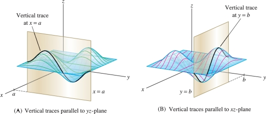
One way of analyzing the graph of a function \(f(x,y)\) is to freeze the \(x\)-coordinate by setting \(x=a\) and examine the resulting curve \(z=f(a,y)\). Similarly, we may set \(y=b\) and consider the curve \(z=f(x,b)\). Curves of this type are called vertical traces. They are obtained by intersecting the graph with planes parallel to a vertical coordinate plane (Figure 14.7):
- Vertical trace in the plane \(x=a\): Intersection of the graph with the vertical plane \(x=a\), consisting of all points \((a,y,f(a,y))\).
- Vertical trace in the plane \(y=b\): Intersection of the graph with the vertical plane \(y=b\), consisting of all points \((x,b,f(x,b))\).
EXAMPLE 3
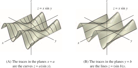
Describe the vertical traces of \(f(x,y)=x\sin y\).
Solution When we freeze the \(x\)-coordinate by setting \(x=a\), we obtain the trace curve \(z = a\sin y\) (see Figure 14.8). This is a sine curve located in the plane \(x=a\). When we set \(y=b\), we obtain a line \(z=(\sin b)y\) of slope \(\sin b\), located in the plane \(y=b\).
777
EXAMPLE 4 Identifying Features of a Graph
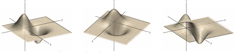
Match the graphs in Figure 14.9 with the following functions:
- (i) \(f(x,y) = x - y^2\)
- (ii) \(g(x,y) = x^2 - y\)
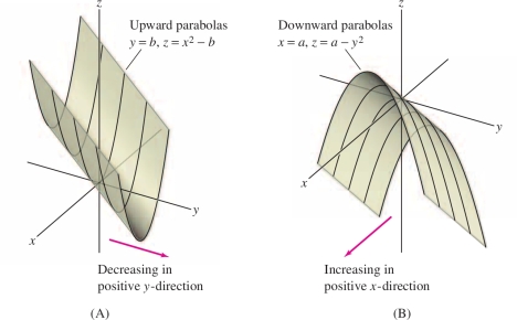
Solution Let’s compare vertical traces. The vertical trace of \(f(x,y) = x - y^2\) in the plane \(x=a\) is a downward parabola \(z=a-y^2\). This matches (B). On the other hand, the vertical trace of \(g(x,y)\) in the plane \(y=b\) is an upward parabola \(z=x^2-b\). This matches (A).
778
Notice also that \(f(x,y)=x-y^2\) is an increasing function of \(x\) (that is, \(f(x,y)\) increases as \(x\) increases) as in (B), whereas \(g(x,y) = x^2 - y\) is a decreasing function of \(y\) as in (A).
Level Curves and Contour Maps
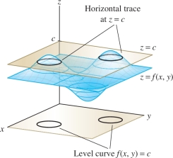
In addition to vertical traces, the graph of \(f(x,y)\) has horizontal traces. These traces and their associated level curves are especially important in analyzing the behavior of the function (Figure 14.10):
- Horizontal trace at height \(c\): Intersection of the graph with the horizontal plane \(z=c\), consisting of the points \((x,y,f(x,y))\) such that \(f(x,y)=c\).
- Level curve: The curve \(f(x,y) = c\) in the \(xy\)-plane.
Thus the level curve consists of all points \((x,y)\) in the plane where the function takes the value \(c\). Each level curve is the projection onto the \(xy\)-plane of the horizontal trace on the graph that lies above it.
A contour map is a plot in the \(xy\)-plane that shows the level curves \(f(x,y) = c\) for equally spaced values of \(c\). The interval \(m\) between the values is called the contour interval. When you move from one level curve to next, the value of \(f(x,y)\) (and hence the height of the graph) changes by \(\pm m\).
On contour maps level curves are often referred to as contour lines.
Figure 14.11 compares the graph of a function \(f(x,y)\) in (A) and its horizontal traces in (B) with the contour map in (C). The contour map in (C) has contour interval \(m = 100\).
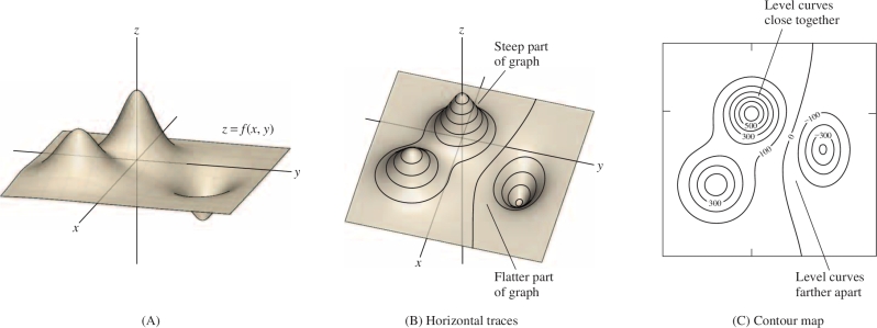
It is important to understand how the contour map indicates the steepness of the graph. If the level curves are close together, then a small move from one level curve to the next in the \(xy\)-plane leads to a large change in height. In other words, the level curves are close together if the graph is steep (Figure 14.11). Similarly, the graph is flatter when the level curves are farther apart.
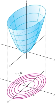
EXAMPLE 5 Elliptic Paraboloid
Sketch the contour map of \(f(x,y)= x^2+3y^2\) and comment on the spacing of the contour curves.
Solution The level curves have equation \(f(x,y)=c\), or \[ x^2+3y^2=c \]
779
- For \(c > 0\), the level curve is an ellipse.
- For \(c=0\), the level curve is just the point \((0,0)\) because \(x^2+3y^2=0\) only for \((x,y)=(0,0)\).
- The level curve is empty if \(c<0\) because \(f(x,y)\) is never negative.
The graph of \(f(x,y)\) is an elliptic paraboloid (Figure 14.12). As we move away from the origin, \(f(x,y)\) increases more rapidly. The graph gets steeper, and the level curves get closer together.
EXAMPLE 6 Hyperbolic Paraboloid
Sketch the contour map of \(g(x,y) = x^2-3y^2\).
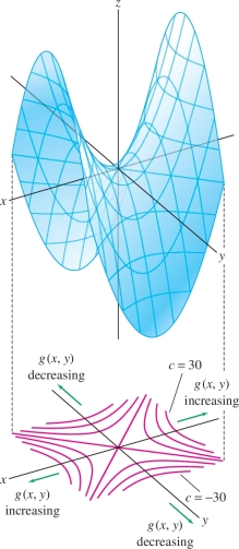
Solution The level curves have equation \(g(x,y)=c\), or \[ x^2-3y^2=c \]
- For \(c \neq 0\), the level curve is the hyperbola \( x^2-3y^2=c\).
- For \(c=0\), the level curve consists of the two lines \(x=\pm \sqrt 3y\) because the equation \(g(x,y) = 0\) factors as follows: \[ x^2-3y^2=0 = (x-\sqrt 3y)(x+\sqrt 3 y) = 0 \]
The graph of \(g(x,y)\) is a hyperbolic paraboloid (Figure 14.13). When you stand at the origin, \(g(x,y)\) increases as you move along the \(x\)-axis in either direction and decreases as you move along the \(y\)-axis in either direction. Furthermore, the graph gets steeper as you move out from the origin, so the level curves get closer together.
REMINDER
The hyperbolic paraboloid in Figure 14.13 is often called a “saddle” or “saddle-shaped surface.”
780
EXAMPLE 7 Contour Map of a Linear Function
Sketch the graph of \(f(x,y) = 12-2x-3y\) and the associated contour map with contour interval \(m=4\).
Solution To plot the graph, which is a plane, we find the intercepts with the axes (Figure 14.14). The graph intercepts the \(z\)-axis at \(z=f(0,0)=12\). To find the \(x\)-intercept, we set \(y=z=0\) to obtain \(12-2x -3(0)=0\), or \(x=6\). Similarly, solving \(12-3y=0\) gives \(y\)-intercept \(y=4\). The graph is the plane determined by the three intercepts.
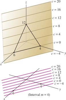
In general, the level curves of a linear function \(f(x,y) =qx + ry + s\) are the lines with equation \(qx + ry + s = c\). Therefore, the contour map of a linear function consists of equally spaced parallel lines. In our case, the level curves are the lines \(12- 2x- 3y= c\), or \(2x+3y=12-c\) (Figure 14.14).
How can we measure steepness quantitatively? Let’s imagine the surface \(z = f(x,y)\) as a mountain range. In fact, contour maps (also called topographical maps) are used extensively to describe terrain (Figure 14.15). We place the \(xy\)-plane at sea level, so that \(f(a,b)\) is the height (also called altitude or elevation) of the mountain above sea level at the point \((a,b)\) in the plane.
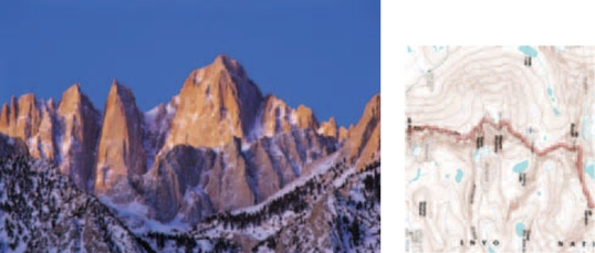
Figure 14.16 shows two points \(P\) and \(Q\) in the \(xy\)-plane, together with the points \(\widetilde P\) and \(\widetilde Q\) on the graph that lie above them. We define the average rate of change: \[ \boxed{\textrm{Average rate of change from }P\textrm{ to }Q =\frac{\Delta \textrm{ altitude}}{\Delta \textrm{ horizontal}}} \]
where
\(\Delta\) altitude \(=\) change in the height from \(\widetilde P\) and \(\widetilde Q\)
\(\Delta\) horizontal \(=\) distance from \(P\) to \(Q\)
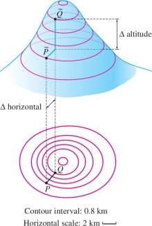
EXAMPLE 8
Calculate the average rate of change of \(f(x,y)\) from \(P\) to \(Q\) for the function whose graph is shown in Figure 14.16.
Solution The segment \(\overline{PQ}\) spans three level curves and the contour interval is \(0.8\) km, so the change in altitude from \(\widetilde P\) to \(\widetilde Q\) is \(3(0.8) = 2.4\) km. From the horizontal scale of the contour map, we see that the horizontal distance \(PQ\) is 2 km, so \[ \textrm{Average rate of change from }P\textrm{ to }Q = \frac{{\rm \Delta} \textrm{ altitude}}{{\rm \Delta} \textrm{ horizontal}} = \frac{2.4}{2} = 1.2 \]
On average, your altitude gain is 1.2 times your horizontal distance traveled as you climb from \(\tilde{P}\) to \(\tilde{Q}\).
781
CONCEPTUAL INSIGHT
We will discuss the idea that rates of change depend on direction when we come to directional derivatives in Section 14.5. In single-variable calculus, we measure the rate of change by the derivative \(f'(a)\). In the multivariable case, there is no single rate of change because the change in \(f(x,y)\) depends on the direction: The rate is zero along a level curve (because \(f(x,y)\) is constant along level curves), and the rate is nonzero in directions pointing from one level curve to the next (Figure 14.17).
EXAMPLE 9 Average Rate of Change Depends on Direction
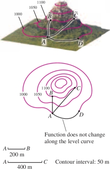
Compute the average rate of change from \(A\) to the points \(B\), \(C\), and \(D\) in Figure 14.17.
Solution The contour interval in Figure 14.17 is \(m=50~\text{m}\). Segments \(\overline{AB}\) and \(\overline{AC}\) both span two level curves, so the change in altitude is 100 m in both cases. The horizontal scale shows that \(AB\) corresponds to a horizontal change of 200 m, and \(\overline{AC}\) corresponds to a horizontal change of 400 m. On the other hand, there is no change in altitude from \(A\) to \(D\). Therefore: \[ \begin{array}{rl} \textrm{Average rate of change from }A\textrm{ to }B &= \frac{\Delta \textrm{ altitude}}{\Delta \textrm{ horizontal}} = \frac{100}{200} = 0.5\\ \textrm{Average rate of change from }A\textrm{ to }C &= \frac{\Delta \textrm{ altitude}}{\Delta \textrm{ horizontal}} = \frac{100}{400} = 0.25 \\ \textrm{Average rate of change from }A\textrm{ to }D &= \frac{\Delta \textrm{ altitude}}{\Delta \textrm{ horizontal}} = 0 \end{array} \]
We see here explicitly that the average rate varies according to the direction.
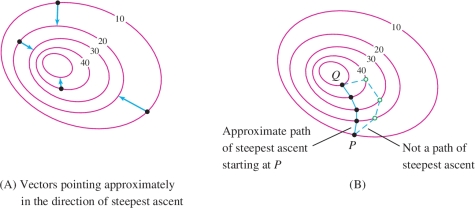
When we walk up a mountain, the incline at each moment depends on the path we choose. If we walk “around” the mountain, our altitude does not change at all. On the other hand, at each point there is a steepest direction in which the altitude increases most rapidly. On a contour map, the steepest direction is approximately the direction that takes us to the closest point on the next highest level curve [Figure 14.18]. We say “approximately” because the terrain may vary between level curves. A path of steepest ascent is a path that begins at a point \(P\) and, everywhere along the way, points in the steepest direction. We can approximate the path of steepest ascent by drawing a sequence of segments that move as directly as possible from one level curve to the next. Figure 14.18 shows two paths from \(P\) to \(Q\). The solid path is a path of steepest ascent, but the dashed path is not, because it does not move from one level curve to the next along the shortest possible segment.
782
A path of steepest descent is the same as a path of steepest ascent but in the opposite direction. Water flowing down a mountain follows a path of steepest descent.
More Than Two Variables
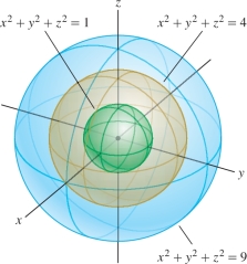
It is not possible to draw the graph of a function of more than two variables. The graph of a function \(f(x,y,z)\) would consist of the set of points \((x,y,z,f(x,y,z))\) in four-dimensional space \({\bf{R}}^4\). However, it is possible to draw the level surfaces of a function of three variables \(f(x,y,z)\). These are the surfaces with equation \(f(x,y,z)=c\). For example, the level surfaces of \[ f(x,y,z)=x^2+y^2+z^2 \] are the spheres with equation \(x^2+y^2+z^2=c\) (Figure 14.19). For functions of four or more variables, we can no longer visualize the graph or the level surfaces. We must rely on intuition developed through the study of functions of two and three variables.
EXAMPLE 10
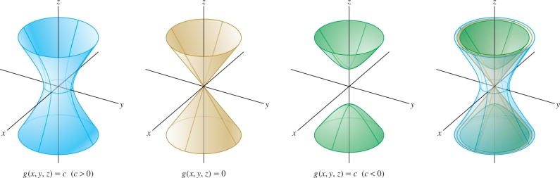
Describe the level surfaces of \(g(x,y,z) = x^2+y^2-z^2\).
Solution The level surface for \(c = 0\) is the cone \(x^2 + y^2 - z^2 = 0\). For \(c \neq 0\), the level surfaces are the hyperboloids \(x^2+y^2-z^2 =c\). The hyperboloid has one sheet if \(c > 0 \) and two sheets if \(c<0\) (Figure 14.20).
14.1.1 Summary
- The domain \({\mathcal{D}}\) of a function \(f(x_1,\dots,x_n)\) of \(n\) variables is the set of \(n\)-tuples \((a_1,\dots,a_n)\) in \({\bf{R}}^n\) for which \(f(a_1,\dots,a_n)\) is defined. The range of \(f\) is the set of values taken by \(f\).
- The graph of a continuous real-valued function \(f(x,y)\) is the surface in \({\bf{R}}^3\) consisting of the points \((a,b,f(a,b))\) for \((a,b)\) in the domain \({\mathcal{D}}\) of \(f\).
- A vertical trace is a curve obtained by intersecting the graph with a vertical plane \(x=a\) or \(y=b\).
- A level curve is a curve in the \(xy\)-plane defined by an equation \(f(x,y) = c\). The level curve \(f(x,y) = c\) is the projection onto the \(xy\)-plane of the horizontal trace curve, obtained by intersecting the graph with the horizontal plane \(z=c\).
- A contour map shows the level curves \(f(x,y) = c\) for equally spaced values of \(c\). The spacing \(m\) is called the contour interval.
- When reading a contour map, keep in mind:
- – Your altitude does not change when you hike along a level curve.
- – Your altitude increases or decreases by \(m\) (the contour interval) when you hike from one level curve to the next.
- The spacing of the level curves indicates steepness: They are closer together where the graph is steeper.
- The average rate of change from \(P\) to \(Q\) is the ratio \(\dfrac{\Delta \textrm{altitude}}{\Delta \textrm{horizontal}}\).
- A direction of steepest ascent at a point \(P\) is a direction along which \(f(x,y)\) increases most rapidly. The steepest direction is obtained (approximately) by drawing the segment from \(P\) to the nearest point on the next level curve.
783