14.2 Limits and Continuity in Several Variables
This section develops limits and continuity in the multivariable setting. We focus on functions of two variables, but similar definitions and results apply to functions of three or more variables.
Recall that a number \(x\) is close to \(a\) if the distance \(|x-a|\) is small. In the plane, one point \((x,y)\) is close to another point \(P = (a,b)\) if the distance between them is small. To express this precisely, we define the open disk of radius \(r\) and center \(P=(a,b)\) (Figure 14.21): \[ \begin{array}{rl} D(P,r) &= \{(x,y)\in{\bf{R}}^2: (x-a)^2+(y-b)^2< r^2\} \end{array} \]
787
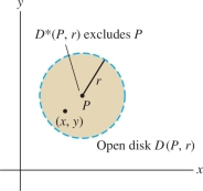
The open punctured disk \(D^*(P,r)\) is the disk \(D(P,r)\) with its center point \(P\) removed. Thus \(D^*(P,r)\) consists of all points whose distance to \(P\) is less than \(r\), other than \(P\) itself.
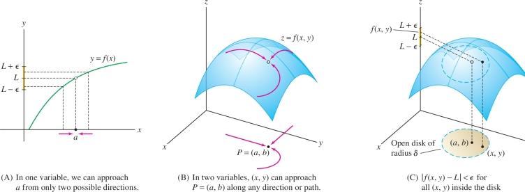
Now assume that \(f(x,y)\) is defined near \(P\) but not necessarily at \(P\) itself. In other words, \(f(x,y)\) is defined for all \((x,y)\) in some punctured disk \(D^*(P,r)\) with \(r>0\). We say that \(f(x,y)\) approaches the limit \(L\) as \((x,y)\) approaches \(P = (a,b)\) if \(|f(x,y)-L|\) becomes arbitrarily small for \((x,y)\) in a sufficiently small punctured disk centered at \(P\) [Figure 14.22]. In this case, we write \[ \lim_{(x,y)\to P}\, f(x,y) = \lim_{(x,y)\to (a,b)}\, f(x,y) = L \]
Here is the formal definition.
DEFINITION Limit
Assume that \(f(x,y)\) is defined near \(P=(a,b)\). Then \[ \lim_{(x,y)\to P} f(x,y) = L \] if, for any \(\epsilon>0\), there exists \(\delta >0\) such that \[ |f(x,y)-L| <\epsilon \quad\textrm{for all}\quad (x,y)\in D^*(P,\delta) \]
This is similar to the limit definition in one variable, but there is an important difference. In a one-variable limit, we require that \(f(x)\) tend to \(L\) as \(x\) approaches \(a\) from the left or right [Figure 14.22]. In a multivariable limit, \(f(x,y)\) must tend to \(L\) no matter how \((x,y)\) approaches \(P\) [Figure 14.22].
EXAMPLE 1
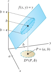
Show that (a) \(\!\!\lim_{(x,y)\to(a,b)} x = a\) and (b) \(\!\!\lim_{(x,y)\to(a,b)} y = b\).
Solution Let \(P=(a,b)\). To verify (a), let \(f(x,y)=x\) and \(L=a\). We must show that for any \(\epsilon >0\), we can find \(\delta>0\) such that \begin{equation} |f(x,y) - L| = |x-a| <\epsilon \quad\textrm{for all}\quad (x,y)\in D^*(P,\delta) \end{equation}
788
In fact, we can choose \(\delta = \epsilon\), for if \((x,y)\in D^*(P,\epsilon)\), then \[ (x-a)^2+(y-b)^2 < \epsilon^2\quad\Rightarrow\quad (x-a)^2< \epsilon^2\quad\Rightarrow\quad |x-a|< \epsilon \]
In other words, for any \(\epsilon > 0\), \[ |x-a| <\epsilon \quad\textrm{for all}\quad (x,y)\in D^*(P,\epsilon) \]
This proves (a). The limit (b) is similar (see Figure 14.23).
The following theorem lists the basic laws for limits. We omit the proofs, which are similar to the proofs of the single-variable Limit Laws.
THEOREM 1 Limit Laws
Assume that \(\lim\limits_{(x,y)\to P} f(x,y)\) and \(\lim\limits_{(x,y)\to P} g(x,y)\) exist. Then:
- (i) Sum Law: \[ \lim_{(x,y)\to P} \left( f(x,y)+g(x,y) \right) = \lim_{(x,y)\to P}f(x,y) + \lim_{(x,y)\to P} g(x,y) \]
- (ii) Constant Multiple Law: For any number \(k\), \[ \lim_{(x,y)\to P} kf(x,y) = k \lim_{(x,y)\to P} f(x,y) \]
- (iii) Product Law: \[ \lim_{(x,y)\to P} f(x,y)\,g(x,y) = \left(\lim_{(x,y)\to P} f(x,y)\right)\left(\lim_{(x,y)\to P} g(x,y)\right) \]
- (iv) Quotient Law: If \(\lim\limits_{(x,y)\to P} g(x,y)\ne 0\), then \[ \lim_{(x,y)\to P} \dfrac{f(x,y)}{g(x,y)} = \dfrac{\lim\limits_{(x,y)\to P} f(x,y)}{\lim\limits_{(x,y)\to P}g(x,y)} \]
As in the single-variable case, we say that \(f\) is continuous at \(P=(a,b)\) if \(f(x,y)\) approaches the function value \(f(a,b)\) as \((x,y)\to (a,b)\).
DEFINITION Continuity
A function \(f(x,y)\) is continuous at \(P=(a,b)\) if \[ \lim_{(x,y)\to(a,b)} f(x,y) = f(a,b) \]
We say that \(f\) is continuous if it is continuous at each point \((a,b)\) in its domain.
The Limit Laws tell us that all sums, multiples, and products of continuous functions are continuous. When we apply them to \(f(x,y)=x\) and \(g(x,y)=y\), which are continuous by Example 1, we find that the power functions \(f(x,y)=x^my^n\) are continuous for all whole numbers \(m, n\) and that all polynomials are continuous. Furthermore, a rational function \(h(x,y)/g(x,y)\), where \(h\) and \(g\) are polynomials, is continuous at all points \((a,b)\) where \(g(a,b)\ne 0\). As in the single-variable case, we can evaluate limits of continuous functions using substitution.
789
EXAMPLE 2 Evaluating Limits by Substitution
Show that \[ f(x,y)=\frac{3x + y}{x^2 + y^2 + 1} \] is continuous (Figure 14.24). Then evaluate \(\lim_{(x,y)\to (1,2)}f(x,y)\).
Solution The function \(f(x,y)\) is continuous at all points \((a,b)\) because it is a rational function whose denominator \(Q(x,y)=x^2 + y^2 + 1\) is never zero. Therefore, we can evaluate the limit by substitution: \[ \lim_{(x,y)\to (1,2)} \frac{3x + y}{x^2 + y^2 + 1} = \frac{3(1)+2}{1^2 + 2^2 + 1} = \frac56 \]
If \(f(x,y)\) is a product \(f(x,y) = h(x)g(y)\), where \(h(x)\) and \(g(y)\) are continuous, then the limit is a product of limits by the Product Law: \[ \lim_{(x,y)\to (a,b)} f(x,y) = \lim_{(x,y)\to (a,b)} h(x)g(y) = \left(\lim_{x\to a} h(x) \right)\left(\lim_{y\to b} g(y)\right) \]
EXAMPLE 3 Product Functions
Evaluate \(\lim_{(x,y)\to (3,0)}\, \,x^3\frac{\sin y}y\).
Solution The limit is equal to a product of limits: \[ \lim_{(x,y)\to (3,0)}\, \,x^3\frac{\sin y}y = \left(\lim_{x\to 3} x^3 \right)\left(\lim_{y\to 0} \frac{\sin y}y\right) = (3^3)(1) = 27 \]
Composition is another important way to build functions. If \(f(x,y)\) is a function of two variables and \(G(u)\) a function of one variable, then the composite \(G\circ f\) is the function \(G(f(x,y))\). According to the next theorem, a composite of continuous functions is again continuous.
THEOREM 2 A Composite of Continuous Functions Is Continuous
If \(f(x,y)\) is continuous at \((a,b)\) and \(G(u)\) is continuous at \(c=f(a,b)\), then the composite function \(G(f(x,y))\) is continuous at \((a,b)\).
EXAMPLE 4
Write \(H(x,y)=e^{-x^2+2y}\) as a composite function and evaluate \[ \lim_{(x,y)\to (1,2)}H(x,y) \]
Solution We have \(H(x,y)=G\circ f\), where \(G(u)=e^u\) and \(f(x,y)=-x^2+2y\). Both \(f\) and \(G\) are continuous, so \(H\) is also continuous and \[ \lim_{(x,y)\to (1,2)} H(x,y) = \lim_{(x,y)\to (1,2)} e^{-x^2+2y} = e^{-(1)^2+2(2)}=e^{3} \]
We know that if a limit \(\lim_{(x,y)\to (a,b)}f(x,y)\) exists and equals \(L\), then \(f(x,y)\) tends to \(L\) as \((x,y)\) approaches \((a,b)\) along any path. In the next example, we prove that a limit does not exist by showing that \(f(x,y)\) approaches different limits along lines through the origin.
790
EXAMPLE 5 Showing a Limit Does Not Exist
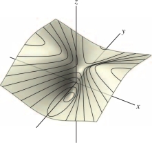
Examine \(\lim_{(x,y)\to (0,0)} \frac{x^2}{x^2+y^2}\) numerically. Then prove that the limit does not exist.
Solution If the limit existed, we would expect the values of \(f(x,y)\) in Table 14.2 to get closer to a limiting value \(L\) as \((x,y)\) gets close to \((0,0)\). But the table suggests that \(f(x,y)\) takes on all values between 0 and 1, no matter how close \((x,y)\) gets to \((0,0)\). For example, \[ f(0.1,0)=1,\qquad f(0.1,0.1)=0.5,\qquad f(0,0.1)=0 \]
Thus, \(f(x,y)\) does not seem to approach any fixed value \(L\) as \((x,y)\to(0,0)\).
Now let’s prove that the limit does not exist by showing that \(f(x,y)\) approaches different limits along the \(x\)- and \(y\)-axes (Figure 14.25): \[ \begin{array}{rl} \textrm{Limit along }x\textrm{-axis:} &\qquad \lim_{x\to 0} f(x,0) = \lim_{x\to 0} \frac{x^2}{x^2+0^2} = \lim_{x\to 0}1= 1 \\ \textrm{Limit along }y\textrm{-axis:} &\qquad \lim_{y\to 0} f(0,y) = \lim_{y\to 0} \frac{0^2}{0^2+y^2} = \lim_{y\to 0} 0 = 0 \end{array} \]
These two limits are different and hence \(\lim_{(x,y)\to (0,0)}f(x,y)\) does not exist.
| \(y\) \ \(x\) | \(-0.5\) | \(-0.4\) | \(-0.3\) | \(-0.2\) | \(-0.1\) | 0 | 0.1 | 0.2 | 0.3 | 0.4 | 0.5 |
| 0.5 | 0.5 | 0.39 | 0.265 | 0.138 | 0.038 | 0 | 0.038 | 0.138 | 0.265 | 0.39 | 0.5 |
| 0.4 | 0.61 | 0.5 | 0.36 | 0.2 | 0.059 | 0 | 0.059 | 0.2 | 0.36 | 0.5 | 0.61 |
| 0.3 | 0.735 | 0.64 | 0.5 | 0.308 | 0.1 | 0 | 0.1 | 0.308 | 0.5 | 0.64 | 0.735 |
| 0.2 | 0.862 | 0.8 | 0.692 | 0.5 | 0.2 | 0 | 0.2 | 0.5 | 0.692 | 0.8 | 0.862 |
| 0.1 | 0.962 | 0.941 | 0.9 | 0.8 | 0.5 | 0 | 0.5 | 0.8 | 0.9 | 0.941 | 0.962 |
| 0 | 1 | 1 | 1 | 1 | 1 | 1 | 1 | 1 | 1 | 1 | |
| \(-0.1\) | 0.962 | 0.941 | 0.9 | 0.8 | 0.5 | 0 | 0.5 | 0.8 | 0.9 | 0.941 | 0.962 |
| \(-0.2\) | 0.862 | 0.8 | 0.692 | 0.5 | 0.2 | 0 | 0.2 | 0.5 | 0.692 | 0.8 | 0.862 |
| \(-0.3\) | 0.735 | 0.640 | 0.5 | 0.308 | 0.1 | 0 | 0.1 | 0.308 | 0.5 | 0.640 | 0.735 |
| \(-0.4\) | 0.610 | 0.5 | 0.360 | 0.2 | 0.059 | 0 | 0.059 | 0.2 | 0.36 | 0.5 | 0.61 |
| \(-\)0.5 | 0.5 | 0.39 | 0.265 | 0.138 | 0.038 | 0 | 0.038 | 0.138 | 0.265 | 0.390 | 0.5 |
GRAPHICAL INSIGHT
The contour map in Figure 14.25 shows clearly that the function \(f(x,y) = {x^2}/({x^2+y^2})\) does not approach a limit as \((x,y)\) approaches \((0,0)\). For nonzero \(c\), the level curve \(f(x,y) = c\) is the line \(y=mx\) through the origin (with the origin deleted) where \(c= (m^2+1)^{-1}\): \[ f(x,mx) =\frac{x^2}{x^2+(mx)^2} = \frac1{m^2+1}\quad(\textrm{for }x\ne 0) \]
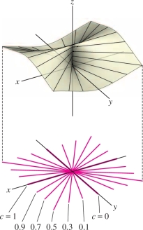
The level curve \(f(x,y) =0\) is the \(y\)-axis (with the origin deleted). As the slope \(m\) varies, \(f\) takes on all values between \(0\) and \(1\) in every disk around the origin \((0,0)\), no matter how small, so \(f\) cannot approach a limit.
As we know, there is no single method for computing limits that always works. The next example illustrates two different approaches to evaluating a limit in a case where substitution cannot be used.
791
EXAMPLE 6 Two Methods for Verifying a Limit
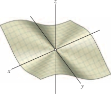
Calculate \(\displaystyle\lim_{(x,y) \to (0,0)} f(x,y)\) where \(f(x,y)\) is defined for \((x,y) \ne (0,0)\) by (Figure 14.26) \[ f(x,y)=\dfrac{xy^2}{x^2+y^2} \]
Solution First Method For \((x,y)\ne (0,0)\), we have \[ 0\le \left| \frac{y^2}{x^2+y^2}\right|\le 1 \] because the numerator is not greater than the denominator. Multiply by \(|x|\): \[ 0 \le \left| \frac{xy^2}{x^2+y^2}\right| \le |x| \] and use the Squeeze Theorem (which is valid for limits in several variables): \[ 0 \le \lim_{(x,y)\to (0,0)}\left|\frac{xy^2}{x^2+y^2}\right| \le \lim_{(x,y)\to (0,0)} |x| \]
Because \(\lim_{(x,y)\to (0,0)} |x| = 0\), we conclude that \(\displaystyle\lim_{(x,y) \to (0,0)} f(x,y)=0\) as desired.
Second Method Use polar coordinates: \[ x = r\cos \theta,\qquad y = r\sin\theta \]
Then \(x^2+y^2 = r^2\) and for \(r \neq 0\), \[ 0 \leq \left|\frac{xy^2}{x^2+y^2}\right| = \left|\frac{(r\cos\theta)(r\sin\theta)^2}{r^2}\right|= r|{\cos\theta\sin^2\theta}|\le r \]
As \((x,y)\) approaches \((0,0)\), the variable \(r\) also approaches \(0\), so again, the desired conclusion follows from the Squeeze Theorem: \[ 0\le \lim_{(x,y)\to (0,0)}\left|\frac{xy^2}{x^2+y^2}\right| \le \lim_{r\to 0}r = 0 \]
14.2.1 Summary
- The open disk of radius \(r\) centered at \(P=(a,b)\) is defined by \[ D(P,r) = \{(x,y)\in{\bf{R}}^2: (x-a)^2+(y-b)^2< r^2\} \] The punctured disk \(D^*(P,r)\) is \(D(P,r)\) with \(P\) removed.
- Suppose that \(f(x,y)\) is defined near \(P=(a,b)\). Then \[ \lim_{(x,y)\to(a,b)} f(x,y) = L \] if, for any \(\epsilon>0\), there exists \(\delta >0\) such that \[ |f(x,y)-L| <\epsilon \quad\textrm{for all}\quad (x,y)\in D^*(P,\delta) \]
- The limit of a product \(f(x,y) = h(x)g(y)\) is a product of limits: \[ \lim_{(x,y)\to (a,b)} f(x,y) = \left(\lim_{x\to a} h(x) \right)\left(\lim_{y\to b} g(y)\right) \]
- A function \(f(x,y)\) is continuous at \(P=(a,b)\) if \[ \lim_{(x,y)\to (a,b)} f(x,y)=f(a,b) \]