14.3 Partial Derivatives
We have stressed that a function \(f\) of two or more variables does not have a unique rate of change because each variable may affect \(f\) in different ways. For example, the current \(I\) in a circuit is a function of both voltage \(V\) and resistance \(R\) given by Ohm’s Law: \[ I(V,R) = \frac{V}R \]
The current \(I\) is increasing as a function of \(V\) but decreasing as a function of \(R\).
The partial derivatives are the rates of change with respect to each variable separately. A function \(f(x,y)\) of two variables has two partial derivatives, denoted \(f_x\) and \(f_y\), defined by the following limits (if they exist): \[ \boxed{\!\!f_x(a,b) = \lim_{h\to 0} \frac{f(a+h,b) - f(a,b)}{h},\quad\,\, f_y(a,b) = \lim_{k\to 0} \frac{f(a,b+k) - f(a,b)}{k}} \]
Thus, \(f_x\) is the derivative of \(f(x,b)\) as a function of \(x\) alone, and \(f_y\) is the derivative at \(f(a,y)\) as a function of \(y\) alone. The Leibniz notation for partial derivatives is \[ \begin{array}{llll} &\frac{\partial f}{\partial x}= f_x,& \quad\qquad &\frac{\partial f}{\partial y}= f_y\\ &\frac{\partial f}{\partial x}\bigg|_{(a,b)} = f_x(a,b),& \quad\qquad &\frac{\partial f}{\partial y}\bigg|_{(a,b)} = f_y(a,b) \end{array} \]
If \(z=f(x,y)\), then we also write \({\partial z}/{\partial x}\) and \({\partial z}/{\partial y}\).
The partial derivative symbol \(\partial\) is a rounded “d.” The symbols \({\partial f}/{\partial x}\) and \({\partial f}/{\partial y}\) are read as follows: “dee-eff dee-ex” and “dee-eff dee-why.”
Partial derivatives are computed just like ordinary derivatives in one variable with this difference: To compute \(f_x\), treat \(y\) as a constant, and to compute \(f_y\), treat \(x\) as a constant.
EXAMPLE 1
Compute the partial derivatives of \(f(x,y) = x^2y^5\).
Solution \[ \begin{array}{rl} \frac{\partial f}{\partial x} &= \underbrace{\frac{\partial}{\partial x} \big(x^2y^5\big)= y^5\frac{\partial}{\partial x} \big(x^2\big)}_{\textrm{Treat }y^5\textrm{ as a constant}} = y^5(2x)=2xy^5 \\ \frac{\partial f}{\partial y} &= \underbrace{\frac{\partial}{\partial y} \big(x^2y^5\big)= x^2\frac{\partial}{\partial x} \big(y^5\big)}_{\textrm{Treat }x^2\textrm{ as a constant}} = x^2(5y^4)=5x^2y^4 \end{array} \]
GRAPHICAL INSIGHT
The partial derivatives at \(P = (a,b)\) are the slopes of the tangent lines to the vertical trace curves through the point \((a,b,f(a,b))\) in Figure 14.27. To compute \(f_x(a,b)\), we set \(y=b\) and differentiate in the \(x\)-direction. This gives us the slope of the tangent line to the trace curve in the plane \(y=b\) [Figure 14.27]. Similarly, \(f_y(a,b)\) is the slope of the trace curve in the vertical plane \(x=a\) [Figure 14.27].

The differentiation rules from calculus of one variable (the Product, Quotient, and Chain Rules) are valid for partial derivatives.
795
EXAMPLE 2
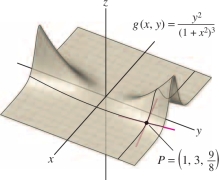
Calculate \(g_x(1,3)\) and \(g_y(1,3)\), where \(g(x,y)=\frac{y^2}{(1+x^2)^3}\).
Solution To calculate \(g_x\), treat \(y\) (and therefore \(y^2\)) as a constant: \[ \begin{array}{rl} g_x(x,y) &= \frac{\partial}{\partial x} \frac{y^2}{(1+x^2)^3} = y^2\frac{\partial}{\partial x} (1+x^2)^{-3}= \frac{-6xy^2}{(1+x^2)^4}\\ g_x(1,3)&= \frac{-6(1)3^2}{(1 + 1^2)^4} = -\frac{27}{8} \end{array} \] To calculate \(g_y\), treat \(x\) (and therefore \(1+x^2\)) as a constant: \begin{equation*} g_y(x,y) = \frac{\partial }{\partial y}\frac{y^2}{(1+x^2)^3} = \frac{1}{(1+x^2)^3}\frac{\partial }{\partial y}y^2 = \frac{2y}{(1+x^2)^3}\tag{1} \end{equation*} \[ g_y(1,3) = \frac{2(3)}{(1 + 1^2)^3} = \frac34 \]
CAUTION
It is not necessary to use the Quotient Rule to compute the partial derivative in Eq. (1). The denominator does not depend on \(y\), so we treat it as a constant when differentiating with respect to \(y\).
These partial derivatives are the slopes of the trace curves through the point \(\big(1,3,\frac98\big)\) shown in Figure 14.28.

We use the Chain Rule to compute partial derivatives of a composite function \(f(x,y)= F(g(x,y))\), where \(F(u)\) is a function of one variable and \(u=g(x,y)\): \[ \frac{\partial f}{\partial x} = \frac{d F}{d u}\frac{\partial u}{\partial x},\qquad \frac{\partial f}{\partial y} = \frac{d F}{d u}\frac{\partial u}{\partial y} \]
EXAMPLE 3 Chain Rule for Partial Derivatives
Compute \(\frac{\partial }{\partial x} \sin(x^2y^5)\).
Solution Write \(\sin(x^2y^5)=F(u)\), where \(F(u)=\sin u\) and \(u=x^2y^5\). Then we have \(\frac{d F}{d u} = \cos u\) and the Chain Rule give us \[ \underbrace{\frac{\partial }{\partial x} \sin(x^2y^5) = \frac{d F}{d u}\frac{\partial u}{\partial x}= \cos(x^2y^5)\frac{\partial }{\partial x}x^2y^5}_{\textrm{Chain Rule}} =2xy^5\cos(x^2y^5) \]
Partial derivatives are defined for functions of any number of variables. We compute the partial derivative with respect to any one of the variables by holding the remaining variables constant.
796
EXAMPLE 4 More Than Two Variables
Calculate \(f_z(0,0,1,1)\), where \[ f(x,y,z,w) = \frac{e^{xz+y}}{z^2+w} \]
Solution Use the Quotient Rule, treating \(x\), \(y\), and \(w\) as constants: \[ \begin{array}{rl} f_z(x,y,z,w) &= \frac{\partial}{\partial z}\left( \frac{e^{xz+y}}{z^2+w}\right) = \frac{(z^2+w)\frac{\partial}{\partial z} e^{xz+y}- e^{xz+y} \frac{\partial}{\partial z}(z^2+w)}{(z^2+w)^2} \\[6pt] &= \frac{(z^2+w)x e^{xz+y}- 2ze^{xz+y}}{(z^2+w)^2} = \frac{(z^2x+wx-2z)e^{xz+y}}{(z^2+w)^2}\\[6pt] f_z(0,0,1,1)&=\frac{-2e^0}{(1^2+1)^2}=-\frac12 \end{array} \]
In Example 4, the calculation \[ \frac{\partial}{\partial z} e^{xz+y}=xe^{xz+y} \] follows from the Chain Rule, just like \[ \frac{d }{d z} e^{az+b}=ae^{az+b} \]
Because the partial derivative \(f_x(a,b)\) is the derivative \(f(x,b)\), viewed as a function of \(x\) alone, we can estimate the change \(\Delta f\) when \(x\) changes from \(a\) to \(a+\Delta x\) as in the single-variable case. Similarly, we can estimate the change when \(y\) changes by \(\Delta y\). For small \(\Delta x\) and \(\Delta y\) (just how small depends on \(f\) and the accuracy required): \[ \boxed{\begin{array}{rcl} f(a+\Delta x,b) -f(a,b)\,\,&\approx&\,\, f_x(a,b)\Delta x \\ \\ f(a,b+\Delta y) -f(a,b)\,\,&\approx&\,\, f_y(a,b)\Delta y \end{array}} \]
This applies to functions \(f\) in any number of variables. For example, \(\Delta f \approx f_w \Delta w\) if one of the variables \(w\) changes by \(\Delta w\) and all other variables remain fixed.
EXAMPLE 5 Testing Microchips
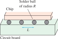
A ball grid array (BGA) is a microchip joined to a circuit board by small solder balls of radius \(R\) mm separated by a distance \(L\) mm (Figure 14.29). Manufacturers test the reliability of BGAs by subjecting them to repeated cycles in which the temperature is varied from \(0^\circ\)C to \(100^\circ\)C over a 40-min period. According to one model, the average number \(N\) of cycles before the chip fails is \[ N = \left(\frac{2200R}{Ld} \right)^{1.9} \] where \(d\) is the difference between the coefficients of expansion of the chip and the board. Estimate the change \(\Delta N\) when \(R=0.12\), \(d = 10\), and \(L\) is increased from 0.4 to 0.42.

Solution We use the approximation \[ \Delta N \approx \frac{\partial N}{\partial L}\,\Delta L \] with \(\Delta L = 0.42-0.4 = 0.02\). Since \(R\) and \(d\) are constant, the partial derivative is \[ \frac{\partial N}{\partial L} = \frac{\partial}{\partial L} \left(\frac{2200R}{Ld} \right)^{1.9} = \left(\frac{2200R}{d} \right)^{1.9}\frac{\partial}{\partial L} L^{-1.9} = -1.9\left(\frac{2200R}{d} \right)^{1.9}L^{-2.9} \]
797
Now evaluate at \(L=0.4\), \(R=0.12\), and \(d=10\): \[ \frac{\partial N}{\partial L}\bigg|_{(L,R,d)=(0.4,0.12,10)} = -1.9\left(\frac{2200(0.12)}{10} \right)^{1.9}(0.4)^{-2.9}\approx -13{,}609 \]
The decrease in the average number of cycles before a chip fails is \[ \Delta N \approx \frac{\partial N}{\partial L}\Delta L =-13{,}609(0.02)\approx -272~\mathrm{cycles} \]
In the next example, we estimate a partial derivative numerically. Since \(f_x\) and \(f_y\) are limits of difference quotients, we have the following approximations when \(h\) and \(k\) are “small”: \[ \boxed{\begin{array}{rcl} f_x(a,b) \,\,&\approx&\,\, \frac{\Delta f}{\Delta x}\,\,=\,\, \frac{f(a+h,b) - f(a,b)}h \\ \\ f_y(a,b)\,\, &\approx&\,\, \frac{\Delta f}{\Delta y}\,\,=\,\, \frac{f(a,b+k) - f(a,b)}k \end{array}} \]
A similar approximation is valid in any number of variables.
EXAMPLE 6 Estimating Partial Derivatives Using Contour Maps
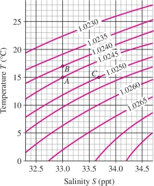
Seawater density \(\rho\) (\(\text{kg/m}^3\)) depends on salinity \(S\) (ppt) and the temperature \(T\) (\(^\circ\)C). Use Figure 14.30 to estimate \({\partial {\rho}}/{\partial T}\) and \({\partial {\rho}}/{\partial {S}}\) at \(A\).

For greater accuracy, we can estimate \(f_x(a,b)\) by taking the average of the difference quotients for \(\Delta x\) and \(-\Delta x\). A similar remark applies to \(f_y(a,b)\).
Solution Point \(A\) has coordinates \((S,T)=(33,15)\) and lies on the level curve \(\rho=1.0245\). We estimate \({\partial {\rho}}/{\partial T}\) at \(A\) in two steps.
Step 1. Move vertically from \(A\).
Since \(T\) varies in the vertical direction, we move up vertically from point \(A\) to point \(B\) on the next higher level curve, where \(\rho = 1.0240\). Point \(B\) has coordinates \((S,T) = (33,17)\). Note that in moving from \(A\) to \(B\), we have kept \(S\) constant because both points have salinity \(S = 33\).
Step 2. Compute the difference quotient
\[ \begin{array}{rl} \Delta \rho &= 1.0240-1.0245=-0.0005\,\,\textrm{kg/m}^3\\ \Delta T &= 17 - 15 = 2^\circ \textrm{C} \end{array} \]
This gives us the approximation \[ \frac{\partial \rho}{\partial T}\bigg|_A \approx \frac{\Delta \rho}{\Delta T} = \frac{-0.0005}{2} = -0.00025~\text{kg-m}^{-3}/{}^\circ\text{C} \]
We estimate \({\partial {\rho}}/{\partial S}\) in a similar way, by moving to the right horizontally to point \(C\) with coordinates \((S,T) \approx (33.7,15)\), where \(\rho = 1.0250\): \[ \frac{\partial \rho}{\partial S}\bigg|_A \approx \frac{\Delta \rho}{\Delta S} =\frac{1.0250-1.0245}{33.7 - 33} = \frac{0.0005}{0.7} \approx 0.0007~\text{kg-m}^{-3}\text{/ppt} \]
798
Higher-Order Partial Derivatives
The higher-order partial derivatives are the derivatives of derivatives. The second-order partial derivatives of \(f\) are the partial derivatives of \(f_x\) and \(f_y\). We write \(f_{xx}\) for the \(x\)-derivative of \(f_x\) and \(f_{yy}\) for the \(y\)-derivative of \(f_y\): \[ f_{xx} = \frac{\partial }{\partial x}\left(\frac{\partial f}{\partial x}\right), \qquad\quad f_{yy} = \frac{\partial }{\partial y}\left(\frac{\partial f}{\partial y}\right) \]
We also have the mixed partials: \[ f_{xy} = \frac{\partial }{\partial y}\left(\frac{\partial f}{\partial x}\right),\qquad f_{yx} = \frac{\partial }{\partial x}\left(\frac{\partial f}{\partial y}\right) \]
The process can be continued. For example, \(f_{xyx}\) is the \(x\)-derivative of \(f_{xy}\), and \(f_{xyy}\) is the \(y\)-derivative of \(f_{xy}\) (perform the differentiation in the order of the subscripts from left to right). The Leibniz notation for higher-order partial derivatives is \[ f_{xx}= \frac{\partial ^2f}{\partial x^2},\qquad f_{xy}= \frac{\partial^2f}{\partial y\partial x},\qquad f_{yx}= \frac{\partial^2f}{\partial x\partial y},\qquad f_{yy}= \frac{\partial ^2f}{\partial y^2} \]
Higher partial derivatives are defined for functions of three or more variables in a similar manner.
EXAMPLE 7
Calculate the second-order partials of \(f(x,y)=x^3+y^2e^x\).
Solution First, we compute the first-order partial derivatives: \[ f_{x}(x,y) =\frac{\partial}{\partial x}\,(x^3+y^2e^x) = 3x^2+y^2e^x,\qquad f_{y}(x,y)= \frac{\partial}{\partial y}\,(x^3+y^2e^x) = 2ye^x \]
Then we can compute the second-order derivatives: \[ \begin{array}{llll} f_{xx}(x,y) &= \frac{\partial }{\partial x}f_x = \frac{\partial }{\partial x}(3x^2+y^2e^x)&\quad f_{yy}(x,y) &= \frac{\partial }{\partial y}f_y = \frac{\partial }{\partial y}2ye^x\\ & = 6x+y^2e^x,&\quad &= 2e^x\\ f_{xy}(x,y) &= \frac{\partial f_x}{\partial y} = \frac{\partial }{\partial y}(3x^2+y^2e^x) &\quad f_{yx}(x,y) &= \frac{\partial f_y}{\partial x} = \frac{\partial }{\partial x} 2ye^x\\ & =2ye^x,&\quad & =2ye^x \end{array} \]
Remember how the subscripts are used in partial derivatives. The notation \(f_{xyy}\) means “first differentiate with respect to \(x\) and then differentiate twice with respect to \(y\).”
EXAMPLE 8
Calculate \(f_{xyy}\) for \(f(x,y)=x^3+y^2e^x\).
Solution By the previous example, \(f_{xy}=2ye^x\). Therefore, \[ f_{xyy} = \frac{\partial }{\partial y}f_{xy} = \frac{\partial }{\partial y} 2ye^x = 2e^x \]
799
Observe in Example 7 that \(f_{xy}\) and \(f_{yx}\) are both equal to \(2ye^x \). It is a pleasant circumstance that the equality \(f_{xy}=f_{yx}\) holds in general, provided that the mixed partials are continuous. See Appendix D for a proof of the following theorem named for the French mathematician Alexis Clairaut (Figure 14.31).

THEOREM 1 Clairaut’s Theorem: Equality of Mixed Partials
If \(f_{xy}\) and \(f_{yx}\) are both continuous functions on a disk \(D\), then \(f_{xy}(a,b) = f_{yx}(a,b)\) for all \((a,b)\in D\). In other words, \[ \boxed{\frac{\partial ^2f}{\partial x\, \partial y} = \frac{\partial ^2f}{\partial y\, \partial x}} \]
The hypothesis of Clairaut’s Theorem, that \(f_{xy}\) and \(f_{yx}\) are continuous, is almost always satisfied in practice, but see Exercise 84 for an example where the mixed partials are not equal.
EXAMPLE 9
Check that \( \frac{\partial^2W}{\partial U\partial T} =\frac{\partial^2W}{\partial T\partial U}\) for \(W = e^{U/T}\).
Solution We compute both derivatives and observe that they are equal: \[ \begin{array}{rclrcl} \frac{\partial W}{\partial T} &=&e^{U/T}\frac{\partial}{\partial T}\left(\frac{U}T\right) = -UT^{-2}e^{U/T}, & \frac{\partial W}{\partial U} &=& e^{U/T}\frac{\partial}{\partial U} \left(\frac{U}T\right) = T^{-1}e^{U/T} \\ \frac{\partial}{\partial U}\frac{\partial W}{\partial T} &=& -T^{-2}e^{U/T}-UT^{-3}e^{U/T}, & \frac{\partial}{\partial T}\frac{\partial W}{\partial U} &=& -T^{-2}e^{U/T}-UT^{-3}e^{U/T} \end{array} \]
Although Clairaut’s Theorem is stated for \(f_{xy}\) and \(f_{yx}\), it implies more generally that partial differentiation may be carried out in any order, provided that the derivatives in question are continuous (see Exercise 75). For example, we can compute \(f_{xyxy}\) by differentiating \(f\) twice with respect to \(x\) and twice with respect to \(y\), in any order. Thus, \[ f_{xyxy} = f_{xxyy} = f_{yyxx} = f_{yxyx} = f_{xyyx}= f_{yxxy} \]
EXAMPLE 10 Choosing the Order Wisely
Calculate the partial derivative \(g_{zzwx}\), where \(g(x,y,z,w) = x^3w^2z^2+\sin\left(\dfrac{xy}{z^2}\right)\).
Solution Let’s take advantage of the fact that the derivatives may be calculated in any order. If we differentiate with respect to \(w\) first, the second term disappears because it does not depend on \(w\): \[ g_w = \frac{\partial }{\partial w}\left(x^3w^2z^2+\sin\left(\frac{xy}{z^2}\right)\right) = 2x^3wz^2 \]
Next, differentiate twice with respect to \(z\) and once with respect to \(x\): \[ \begin{array}{rl} g_{wz} &= \frac{\partial }{\partial z}2x^3wz^2 = 4x^3wz\\ g_{wzz} &= \frac{\partial }{\partial z}4x^3wz = 4x^3w \\ g_{wzzx} &= \frac{\partial }{\partial x}4x^3w = 12x^2w \end{array} \]
We conclude that \(g_{zzwx} = g_{wzzx} = 12x^2w\).
800
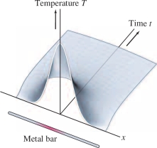
A partial differential equation (PDE) is a differential equation involving functions of several variables and their partial derivatives. The heat equation in the next example is a PDE that models temperature as heat spreads through an object. There are infinitely many solutions, but the particular function in the example describes temperature at times \(t>0\) along a metal rod when the center point is given a burst of heat at \(t=0\) (Figure 14.32).

EXAMPLE 11 The Heat Equation
Show that \(\smash{u(x,t)=\frac1{2\sqrt{\pi t}}e^{-(x^2/4t)}}\), defined for \(t>0\), satisfies the heat equation \begin{equation*} \frac{\partial u}{\partial t} = \frac{\partial^2u}{\partial x^2}\tag{2} \end{equation*}
Solution First, compute \(\smash{\frac{\partial ^2u}{\partial x^2}}\): \[ \begin{array}{llll} \frac{\partial u}{\partial x}&=\frac{\partial}{\partial x}\, \frac1{2\sqrt{\pi}}\,t^{-1/2}e^{-(x^2/4t)}& =&\;{-} \frac1{4\sqrt{\pi}}\,xt^{-3/2} e^{-(x^2/4t)}\\ \frac{\partial ^2u}{\partial x^2}&=\frac{\partial}{\partial x} \left(- \frac1{4\sqrt{\pi}}\, xt^{-3/2}e^{-(x^2/4t)}\right)\,& =&\;{-} \frac{1}{4\sqrt{\pi}}\,t^{-3/2}e^{-(x^2/4t)}+\frac1{8\sqrt{\pi}}\,x^2t^{-5/2}e^{-(x^2/4t)} \end{array} \]
Then compute \({\partial {u}}/{\partial {t}}\) and observe that it equals \({\partial {^2u}}/{\partial {x^2}}\) as required: \[ \frac{\partial u}{\partial t}=\frac{\partial}{\partial t}\left(\frac1{2\sqrt{\pi}}\,t^{-1/2}e^{-(x^2/4t)}\right) = -\frac1{4\sqrt{\pi}}\, t^{-3/2} e^{-(x^2/4t)}+\frac1{8\sqrt{\pi}}\,x^2t^{-5/2} e^{-(x^2/4t)} \]
14.3.1 Summary
- The partial derivatives of \(f(x,y)\) are defined as the limits \[ \begin{array}{rl} f_x(a,b) &=\frac{\partial f}{\partial x}\bigg|_{(a,b)} = \lim_{h\to 0} \frac{f(a+h,b) - f(a,b)}{h}\\ f_y(a,b) &=\frac{\partial f}{\partial y}\bigg|_{(a,b)} = \lim_{k\to 0} \frac{f(a,b+k) -f(a,b)}{k} \end{array} \]
- Compute \(f_x\) by holding \(y\) constant, and compute \(f_y\) by holding \(x\) constant.
- \(f_x(a,b)\) is the slope at \(x=a\) of the tangent line to the trace curve \(z=f(x,b)\). Similarly, \(f_y(a,b)\) is the slope at \(y=b\) of the tangent line to the trace curve \(z=f(a,y)\).
- For small changes \(\Delta x\) and \(\Delta y\), \[ \begin{array}{rcl} f(a+\Delta x,b) -f(a,b)\,\,&\approx&\,\, f_x(a,b)\Delta x \\[6pt] f(a,b+\Delta y) -f(a,b)\,\,&\approx&\,\, f_y(a,b)\Delta y \end{array} \] More generally, if \(f\) is a function of \(n\) variables and \(w\) is one of the variables, then \(\Delta f \approx f_w \Delta w\) if \(w\) changes by \(\Delta w\) and all other variables remain fixed.
- The second-order partial derivatives are \[ \frac{\partial ^2}{\partial x^2}f = f_{xx}, \qquad \frac{\partial ^2}{\partial y\,\partial x}f = f_{xy} , \qquad \frac{\partial ^2}{\partial x\,\partial y}f = f_{yx},\qquad \frac{\partial ^2}{\partial y^2}f = f_{yy} \]
- Clairaut’s Theorem states that mixed partials are equal—that is, \(f_{xy}=f_{yx}\) provided that \(f_{xy}\) and \(f_{yx}\) are continuous.
- More generally, higher-order partial derivatives may be computed in any order. For example, \(f_{xyyz}=f_{yxzy}\) if \(f\) is a function of \(x, y, z\) whose fourth-order partial derivatives are continuous.
801
HISTORICAL PERSPECTIVE


The general heat equation, of which Eq. (2) is a special case, was first introduced in 1807 by French mathematician Jean Baptiste Joseph Fourier. As a young man, Fourier was unsure whether to enter the priesthood or pursue mathematics, but he must have been very ambitious. He wrote in a letter, “Yesterday was my 21st birthday, at that age Newton and Pascal had already acquired many claims to immortality.” In his twenties, Fourier got involved in the French Revolution and was imprisoned briefly in 1794 over an incident involving different factions. In 1798, he was summoned, along with more than 150 other scientists, to join Napoleon on his unsuccessful campaign in Egypt.
Fourier’s true impact, however, lay in his mathematical contributions. The heat equation is applied throughout the physical sciences and engineering, from the study of heat flow through the earth’s oceans and atmosphere to the use of heat probes to destroy tumors and treat heart disease.
Fourier also introduced a striking new technique—known as the Fourier transform—for solving his equation, based on the idea that a periodic function can be expressed as a (possibly infinite) sum of sines and cosines. Leading mathematicians of the day, including Lagrange and Laplace, initially raised objections because this technique was not easy to justify rigorously. Nevertheless, the Fourier transform turned out to be one of the most important mathematical discoveries of the nineteenth century. A Web search on the term “Fourier transform” reveals its vast range of modern applications.
In 1855, the German physiologist Adolf Fick showed that the heat equation describes not only heat conduction but also a wide range of diffusion processes, such as osmosis, ion transport at the cellular level, and the motion of pollutants through air or water. The heat equation thus became a basic tool in chemistry, molecular biology, and environmental science, where it is often called Fick’s Second Law.